The Springer Correspondence, Part III: Hall-Littlewood Polynomials

This is the third post in a series on the Springer correspondence. See Part I and Part II for background.

In this post, we’ll restrict ourselves to the type A setting, in which $\DeclareMathOperator{\GL}{GL}\DeclareMathOperator{\inv}{inv} G=\GL_n(\mathbb{C})$, the Borel $B$ is the subgroup of invertible upper triangular matrices, and $U\subset G$ is the unipotent subvariety. In this setting, the flag variety is isomorphic to $G/B$ or $\mathcal{B}$ where $\mathcal{B}$ is the set of all subgroups conjugate to $B$.

The Hall-Littlewood polynomials

For a given partition $\mu$, the Springer fiber $\mathcal{B}_\mu$ can be thought of as the set of all flags $F$ which are fixed by left multiplication by a unipotent element $u$ of Jordan type $\mu$. In other words, it is the set of complete flags \[F:0=F_0\subset F_1 \subset F_2 \subset \cdots \subset F_n=\mathbb{C}^n\] where $\dim F_i=i$ and $uF_i=F_i$ for all $i$.

In the last post we saw that there is an action of the Weyl group, in this case the symmetric group $S_n$, on the cohomology rings $H^\ast(\mathcal{B}_\mu)$ of the Springer fibers. We let $R_\mu=H^\ast(\mathcal{B}_\mu)$ denote this ring, and we note that its graded Frobenius characteristic \[\DeclareMathOperator{\Frob}{Frob}\widetilde{H}_\mu(X;t):=\Frob_t(H^\ast(\mathcal{B}_\mu))=\sum_{d\ge 0}t^d \Frob(H^{2d}(\mathcal{B}_\mu))\] encodes all of the data determining this ring as a graded $S_n$-module. The symmetric functions $\widetilde{H}_\mu(X,t)\in \Lambda_{\mathbb{Q}(t)}(x_1,x_2,\ldots)$ are called the Hall-Littlewood polynomials.

The first thing we might ask about a Hall-Littlewood polynomial $H_\mu$ is: what is its degree as a polynomial in $t$? In other words…

What is the dimension of $\mathcal{B}_\mu$?

The dimension of $\mathcal{B}_\mu$ will tell us the highest possible degree of its cohomology ring, giving us at least an upper bound on the degree of $H_\mu$. To compute the dimension, we will decompose $\mathcal{B}_\mu$ into a disjoint union of subvarieties whose dimensions are easier to compute.

Let’s start with a simple example. If $\mu=(1,1,1,\ldots,1)$ is a single-column shape of size $n$, then $\mathcal{B}_\mu$ is the full flag variety $\mathcal{B}$, since here the unipotent element $1$ is in the conjugacy class of shape $\mu$, and we can interpret $\mathcal{B}_\mu$ as the set of flags fixed by the identity matrix (all flags). As described in Part I, the flag variety can be decomposed into Schubert cells $X_w$ where $w$ ranges over all permutations in $S_n$ and $\dim(X_w)=\inv(w)$. For instance, $X_{45132}$ is the set of flags defined by the initial row spans of a matrix of the form: \[\left(\begin{array}{ccccc} 0 & 1 & \ast & \ast & \ast \\ 1 & 0 & \ast & \ast & \ast \\ 0 & 0 & 0 & 0 & 1 \\ 0 & 0 & 1 & \ast & 0 \\ 0 & 0 & 0 & 1 & 0 \end{array}\right)\] because this matrix has its leftmost $1$’s in positions $4,5,1,3,2$ from the right in that order.

Thus the dimension of the flag variety is the maximum of the dimensions of these cells. The number of inversions in $w$ is maximized when $w=w_0=n(n-1)\cdots 2 1$, and so \[\dim(\mathcal{B})=\inv(w_0)=\binom{n}{2}.\]

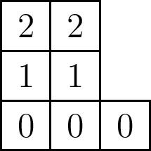
We claim that in general, $\dim(\mathcal{B}_\mu)=n(\mu)$ where if $\mu^\ast$ denotes the conjugate partition, $n(\mu)=\sum \binom{\mu^\ast_i}{2}$. Another way of defining $n(\mu)$ is as the sum of the entries of the superstandard tableau formed by filling the bottom row of $\mu$ with $0$’s, the next row with $1$’s, and so on:

To show this, notice that since $\mathcal{B}_\mu$ is a subvariety of the full flag variety $\mathcal{B}$, and so \[\mathcal{B}_\mu=\mathcal{B}_\mu\cap \mathcal{B}=\bigsqcup \mathcal{B}_\mu\cap X_{w}.\] It thus suffices to find the largest possible dimension of the varieties $\mathcal{B}_\mu\cap X_{w}$.

Let $u$ be the standard unipotent element of Jordan type $\mu$. For instance, the matrix below is the standard unipotent matrix of shape $(3,2,2)$.

Then the set $\mathcal{B}_\mu\cap X_{w}$ can be defined as the subset of $n\times n$ matrices defining flags in $X_w$ whose partial row spans are fixed by the action of $u$. Note that since the first vector is fixed by $u$, it must be equal to a linear combination of the unit vectors $e_{\mu_1}, e_{\mu_1+\mu_2},\ldots$. So we instantly see that the dimension of $\mathcal{B}_\mu\cap X_w$ is in general less than that of $X_w$.

Now, consider the permutation \[\hat{w}=n,n-\mu_1,n-\mu_1-\mu_2,\ldots,n-1,n-1-\mu_1,n-1-\mu_1-\mu_2,\ldots,\ldots.\] Then it is not hard to see that the matrices in $X_{\hat{w}}$ whose flags are fixed by $u$ are those with $1$’s in positions according to $\hat{w}$, and with $0$’s in all other positions besides those in row $i$ from the top and column $k-\mu_1-\cdots-\mu_j$ from the right for some $i,j,k$ satisfying $i\le j$ and $\mu^\ast_1+\cdots+\mu^\ast_k< i \le \mu^\ast_1+\cdots+\mu^\ast_{k+1}$.

This is a mouthful which is probably better expressed via an example. If $\mu=(3,2,2)$ as above, then $\hat{w}=7426315$, and $\mathcal{B}_\mu\cap X_{7426315}$ is the set of flags determined by the rows of matrices of the form \[\left(\begin{array}{ccccccc} 1 & 0 & 0 & \ast & 0 & \ast & 0 \\ 0 & 0 & 0 & 1 & 0 & \ast & 0 \\ 0 & 0 & 0 & 0 & 0 & 1 & 0 \\ 0 & 1 & 0 & 0 & \ast & 0 & \ast \\ 0 & 0 & 0 & 0 & 1 & 0 & \ast \\ 0 & 0 & 0 & 0 & 0 & 0 & 1 \\ 0 & 0 & 1 & 0 & 0 & 0 & 0 \\ \end{array}\right)\]

The first three rows above correspond to the first column of $\mu$, the next three rows to the second column, and the final row to the last column. Notice that the stars in each such block of rows form a triangular pattern similar to that for $X_{w_0}$, and therefore there are $n(\mu)=\binom{\mu^\ast_1}{2}+\binom{\mu^\ast_2}{2}+\cdots$ stars in the diagram. Thus $\mathcal{B}_\mu\cap X_{\hat{w}}$ an open affine set of dimension $n(\mu)$, and so $\mathcal{B}_\mu$ has dimension at least $n(\mu)$.

A bit more fiddling with linear algebra and multiplication by $u$ (try it!) shows that, in fact, for any permutation $w$, the row with a $1$ in the $i$th position contributes at most as many stars in $\mathcal{B}_\mu\cap X_{w}$ as it does in $\mathcal{B}_\mu\cap X_{\hat{w}}$. In other words, all other components $\mathcal{B}_\mu\cap X_{w}$ have dimension at most $n(\mu)$, and so \[\dim\mathcal{B}_\mu=n(\mu).\]

The orthogonality relations

In Lusztig’s survey on character sheaves, he shows that the Hall-Littlewood polynomials (and similar functions for other Lie types) satisfy certain orthogonality and triangularity conditions that determine them completely. To state them in the type A case, we first define $\widetilde{H}_\mu[(1-t)X;t]$ to be the result of plugging in the monomials $x_1,-tx_1,x_2,-tx_2,\ldots$ for $x_1,x_2,\ldots$ in the Hall-Littlewood polynomials. (This is a special kind of plethystic substitution.) Then Lusztig’s work shows that:

• $\left\langle \widetilde{H}_\mu(X;t),s_\lambda\right\rangle=0$ for any $\lambda<\mu$ in dominance order, and $\langle\widetilde{H}_\mu,s_\mu\rangle=1$

• $\left\langle \widetilde{H}_\mu[(1-t)X;t],s_\lambda\right\rangle=0$ for any $\lambda>\mu$ in dominance order

• $\left\langle \widetilde{H}_\mu(X;t),\widetilde{H}_{\lambda}[(1-t)X;t]\right\rangle=0$ whenever $\lambda\neq \mu$.

In all three of the above, the inner product $\langle,\rangle$ is the Hall inner product, which can be defined as the unique inner product for which \[\langle s_\lambda,s_\mu\rangle = \delta_{\lambda\mu}\] for all $\lambda$ and $\mu$.

Since the Schur functions $s_\lambda$ correspond to the irreducible representations $V_\lambda$ of $S_n$, we can therefore interpret these orthogonality conditions in a representation theoretic manner. The inner product $\left \langle \widetilde{H}_\mu(X;t),s_\lambda \right\rangle$ is the coefficient of $s_\lambda$ in the Schur expansion of $\widetilde{H}_\mu$, and is therefore the Hilbert series of the isotypic component of type $V_\lambda$ in the cohomology ring $R_\mu=H^\ast(\mathcal{B}_\mu)$. Moreover, the seemingly arbitrary substitution $X\mapsto (1-t)X$ actually corresponds to taking tensor products with the exterior powers of the permutation representation $V$ of $S_n$. To be precise: \[\widetilde{H}_\mu[(1-t)X;t]=\sum_{i\ge 0} (-1)^i t^i \Frob_t(R_\mu\otimes \Lambda^i(V)).\]

It turns out that any two of the three conditions above uniquely determine the Hall-Littlewood polynomials, and in fact can be used to calculate them explicitly. We now work out an example using the first and third conditions above.

Example: $n=3$

As an example, let’s calculate the Hall-Littlewood polynomials whose partition $\mu$ has size $n=3$. That is, we wish to find $\widetilde{H}_{(3)}$, $\widetilde{H}_{(2,1)}$, and $\widetilde{H}_{(1,1,1)}$. In particular let’s try to find their explicit expansions in terms of Schur functions.

To work out this example, I took out my new Microsoft Surface and its magnetic tablet pen, and by the time I was done with the entire calculation, it looked like this:

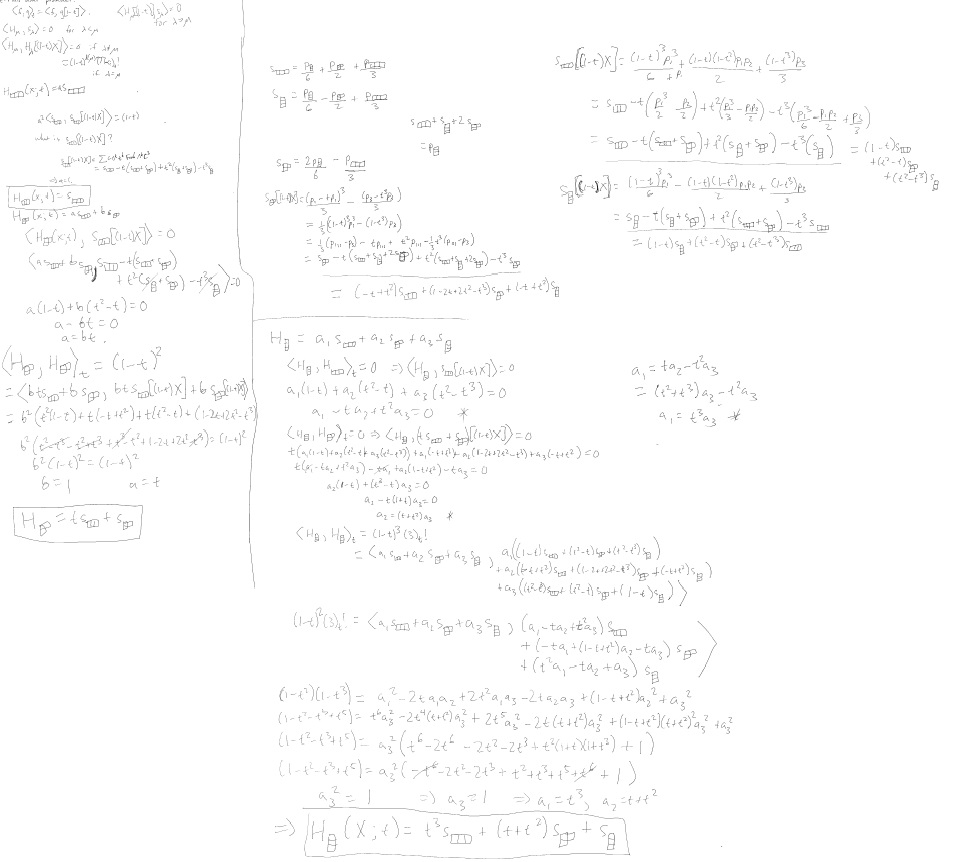
It’s a long slog that is better done by computer, so I’ll just provide a summary of the calculation with some of the main details. Recall that we are working with the conditions:

1. $\left\langle \widetilde{H}_\mu(X;t),s_\lambda\right\rangle=0$ for any $\lambda<\mu$ in dominance order, and $\langle\widetilde{H}_\mu,s_\mu\rangle=1$
2. $\left\langle \widetilde{H}_\mu(X;t),\widetilde{H}_{\lambda}[(1-t)X;t]\right\rangle=0$ whenever $\lambda\neq \mu$.

We can start by finding $\widetilde{H}_{(3)}$, which cannot have any $s_{(2,1)}$’s or $s_{(1,1,1)}$’s in its expansion by condition (1) above. So \[\widetilde{H}_{(3)}=a\cdot s_{(3)}\] for some $a\in \mathbb{Q}(t)$. In fact, the diagonal condition in (1) says that $a=1$, so we have \[\widetilde{H}_{(3)}=s_{(3)}.\]

To find $\widetilde{H}_{(2,1)}$, we first use condition (1) to find that we can express it as \[\widetilde{H}_{(2,1)}=s_{(2,1)}+b\cdot s_{(3)}\] for some $b\in \mathbb{Q}(t)$. Furthermore, by condition (2), it must be orthogonal to $\widetilde{H}_{(3)}[(1-t)X;t]$. So we now need to understand $\widetilde{H}_\mu[(1-t)X;t]$. This is equal to $s_{(3)}[(1-t)X]$, and so it suffices to understand what the substitution $X\mapsto (1-t)X$ does to Schur functions.

To make this substitution, we first express them in terms of the power sum symmetric functions and then make the substitution on each. The character table for $S_3$ is: \[\begin{array}{c|ccc} & [(1)(2)(3)] & [(12)(3)] & [(123)] \\\hline \chi^{(3)} & 1 & 1 & 1 \\ \chi^{(1,1,1)} & 1 & -1 & 1 \\ \chi^{(2,1)} & 2 & 0 & -1 \end{array} \] Using the formula $s_\lambda=\sum \frac{1}{z_\mu} \chi^\lambda(\mu)p_\mu$ where $z_\mu=\prod i^\alpha_i\alpha_i!$ and $\alpha_i$ is the number of times $i$ occurs in $\mu$, we have

• $s_{(3)}=\frac{p_{(1,1,1)}}{6}+\frac{p_{(2,1)}}{2}+\frac{p_{(3)}}{3}$
• $s_{(1,1,1)}=\frac{p_{(1,1,1)}}{6}-\frac{p_{(2,1)}}{2}+\frac{p_{(3)}}{3}$
• $s_{(2,1)}=\frac{p_{(1,1,1)}}{3}-\frac{p_{(3)}}{3}$

Notice that plugging in $x_1,-tx_1,x_2,-tx_2,\ldots$ into a power sum symmetric function $p_{k}$ yields $p_k-t^kp_k=(1-t^k)p_k$, so we have \[p_\mu[(1-t)X]=p_\mu\cdot \prod (1-t^{\mu_i}).\] Thus \[s_{(3)}[(1-t)X]=(1-t)^3\frac{p_{(1,1,1)}}{6}+(1-t^2)(1-t)\frac{p_{(2,1)}}{2}+(1-t^3)\frac{p_{(3)}}{3},\] and we can use the equations above to convert this back into a sum of Schur functions: \[\begin{eqnarray*} s_{(3)}[(1-t)X] &=& s_{(3)}-t(s_{(3)}+s_{(2,1)})+t^2(s_{(1,1,1)}+s_{(2,1)})-t^3s_{(1,1,1)} \\ &=& (1-t)s_{(3)}+(t^2-t)s_{(2,1)}+(t^2-t^3)s_{(1,1,1)} \end{eqnarray*}\] We can now finish the computation of $\widetilde{H}_{(2,1)}(X;t)$. The orthogonality relation says that \[\langle s_{(2,1)}+b\cdot s_{(3)}, s_{3}[(1-t)X]\rangle=0.\] By the expansion of $s_{(3)}[(1-t)X]$ above and using the orthogonality of the Schur functions, the left hand side becomes $(t^2-t)+b(1-t)$. Thus $b(1-t)=t-t^2$, and so $b=t$. It follows that \[\widetilde{H}_{(2,1)}(X;t)=s_{(2,1)}+ts_{(3)}.\]

Finally, a similar calculation shows that \[\widetilde{H}_{(1,1,1)}(X;t)=s_{(1,1,1)}+(t+t^2)s_{(2,1)}+t^3s_{(3)}.\]

Indeed, the degree of these polynomials $\widetilde{H}_\mu(X;t)$ as a polynomial in $t$ is equal to $n(\mu)$ in each case above.

The Cocharge Formula

A similar method can be used to compute the characters of the $W$-modules $H^\ast(\mathcal{B}_u)$ for any Lie type. In type A, however, there is a much simpler formula for the Hall-Littlewood polynomials. It is based on a combinatorial statistic on semistandard Young tableaux called cocharge. We write $\DeclareMathOperator{\cc}{cc}\cc(T)$ to denote the cocharge of a tableau $T$.

Let $\widetilde{K_{\lambda\mu}}(t)$ denote the coefficient of $s_\lambda$ in $\widetilde{H}_\mu(X;t)$, so in other words \[\widetilde{H}_\mu(X;t)=\sum_{\lambda} \widetilde{K_{\lambda\mu}}(t) s_\lambda.\] Since the Hall-Littlewood polynomials are the Frobenius characteristic of a graded $S_n$-module, we know that $\widetilde{K_{\lambda\mu}}(t)$ is always a polynomial in $t$ with positive integer coefficients. In fact we have \[\widetilde{K_{\lambda\mu}}(t)=\sum_{T\in SSYT(\lambda,\mu)}t^{\cc(T)}\] where $SSYT(\lambda,\mu)$ denotes the set of all semistandard Young tableaux of shape $\lambda$ and content $\mu$. That is, $T$ ranges over all fillings of the diagram of $\lambda$ that are weakly increasing along rows and strictly increasing up columns, and use exactly $\mu_i$ copies of the entry $i$ for each $i$.

To define the cocharge of such a filling, we define a cocharge statistic on words having partition content, and then simply define $\cc(T)$ to be the cocharge of its reading word. Given a word $w=w_1\cdots w_n$ of content $\mu$, we decompose it into standard subwords $w^{(1)},\ldots,w^{(\mu_1)}$ as follows. Search from the right until you find a $1$, then continue until finding a $2$, and so on, possibly wrapping around to the beginning if you reach the left end of the word, and stopping when a copy of the largest letter in the word is found. Then these letters form the subword $w^{(1)}$. We then remove $w^{(1)}$ and repeat the process on the remaining word to find $w^{(2)}$ and so on.

Now, for a standard subword $w^{(k)}$, let $a_i$ be the number of times we wrapped around the left edge of $w$ in our search before arriving at the entry $i$ in $w^{(k)}$. We define \[\cc(w^{(k)})=\sum_i i-1-a_i,\] and define \[\cc(w)=\cc(w^{(1)})+\cdots+\cc(w^{(\mu_1)}).\]

For instance, if \[w=13224121353,\] then our standard subwords are $w^{(1)}=34215$, $w^{(2)}=213$, and $w^{(3)}=123$. The cocharge of $w^{(1)}$ is the sum of the subscripts in the labeling \[3_2 4_2 2_1 1_0 5_2,\] since we had to wrap around once to find the $4$ and a total of twice to find the $5$. So $\cc(w^{(1)})=7$, $\cc(w^{(2)})=2$, and $\cc(w^{(3)})=0$. Hence $\cc(w)=7+2=9$.

Finally, the cocharge of a tableau is the cocharge of its reading word. So to compute, say, $\widetilde{K}_{(1,1,1),(2,1)}(t)$, we consider the two semistandard fillings of shape $(2,1)$ and content $(1,1,1)$:

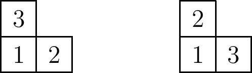
Their reading words are $213$ and $312$, which have cocharge $2$ and $1$ respectively. Hence \[\widetilde{K}_{(1,1,1),(2,1)}(t)=t+t^2.\] Notice that this is indeed the coefficient of $s_{(2,1)}$ in $\widetilde{H}_{(1,1,1)}(X;t)$ that we found above by orthogonality!

Finally, it also follows immediately from this formula that the degree of $\widetilde{H}_\mu(X;t)$ is $n(\mu)$. Indeed, it is the cocharge of the superstandard filling

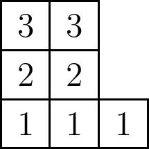
We know it is maximal, since the cocharge of a filling with content $\mu$ is maximized when the number of times we wrap around the left edge to find each standard subword is minimized. Since there is no wrapping around at all in the reading word of the superstandard filling, it follows that $n(\mu)$ is the degree of $\widetilde{H}_\mu(X;t)$.