The CW complex structure of the Grassmannian

In a previous post, we briefly described the complex Grassmannian $\mathrm{Gr}(n,k)$ as a CW complex whose cells are the Schubert cells with respect to a chosen flag. We’ll now take a closer look at the details of this construction, along the lines of the exposition in this master’s thesis of Tuomas Tajakka (chapter 3) or Hatcher’s book Vector Bundles and $K$-theory (page 31), but with the aid of concrete examples.

Background on CW complexes

Let’s first review the notion of a CW complex (or cell complex), as described in Hatcher’s Algebraic Topology.

An $n$-cell is any topological space homeomorphic to the open ball $B_n=\{v\in\mathbb{R}^n:|v|<1\}$ in $\mathbb{R}^n$. Similarly an $n$-disk is a copy of the closure $\overline{B_n}=\{v\in \mathbb{R}^n:|v|\le 1\}$.

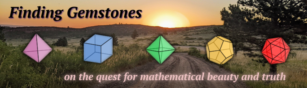
To construct a cell complex, one starts with a set of points called the $0$-skeleton $X^0$, and then attaches $1$-disks $D$ via continuous boundary maps from the boundary $\partial D$ (which simply consists of two points) to $X^0$. The result is a $1$-skeleton $X^1$, which essentially looks like a graph:

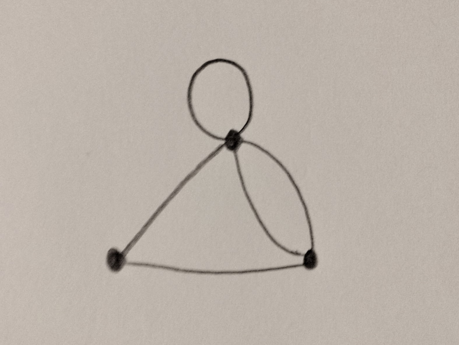
This can then be extended to a $2$-skeleton by attaching $2$-disks $D$ via maps from the boundary $\partial D$ (which is a circle) to $X^1$. Note that, as in the picture below, the attaching map may collapse the entire boundary to a point, making the circle into a balloon-like shape.

In general the $n$-skeleton $X^n$ is formed from $X^{n-1}$ by attaching a set of $n$-disks by maps from their boundaries to $X^{n-1}$.

More precisely, to form $X^n$ from $X^{n-1}$, we start with a collection of $n$-disks $D^n_\alpha$ and continuous attaching maps $\varphi_\alpha:\partial D_\alpha^n\to X^{n-1}$. Then \[X^n=\frac{X^{n-1}\sqcup \bigsqcup_\alpha D_\alpha^n}{\sim}\] where $\sim$ is the identification $x\sim \varphi_\alpha(x)$ for $x\in \partial D^n_\alpha$. The cell complex is $X=\bigcup_n X^n$, which may be simply $X=X^n$ if the process stops at stage $n$.

By the construction, the points $X^0$ along with the open $i$-cells associated to the $i$-disks in $X^i$ for each $i$ are disjoint and cover the cell complex $X$. The topology on $X$ is given by the rule that $A\subset X$ is open if and only if $A\cap X^n$ is open in $X^n$ for all $n$.

The real projective plane

As an example, consider the real projective plane $\mathbb{P}^2_{\mathbb{R}}$. It has a cell complex structure in which $X^0=\{(0:0:1)\}$ is a single point, and $X^1=X^0\sqcup \{(0:1:\ast)\}$ is topologically a circle formed by attaching a $1$-cell to the point at both ends.

Then, $X^2$ is formed by attaching a $2$-cell $\mathbb{R}^2$ to the circle such that the boundary wraps around the $1$-cell twice. Intuitively, this is because the points of the form $(1:xt:yt)$ as $t\to \infty$ and as $t\to -\infty$ both approach the same point in $X^1$, so the boundary map must be a $2$-to-$1$ mapping.

To make this analysis more rigorous, consider $\mathbb{P}^2_{\mathbb{R}}$ as the quotient $(\mathbb{R}^3\setminus\{(0,0,0)\})/\sim$ where $\sim$ is the equivalence relation given by scalar multiplication. In particular there is a natural continuous quotient map \[q:\mathbb{R}^3\setminus \{0\}\to \mathbb{P}^2_{\mathbb{R}}.\] We can now take $n$-disks in $\mathbb{R}^3\setminus\{0\}$ and map them into $\mathbb{P}^2_{\mathbb{R}}$ via $q$, which will give the CW complex structure described above.

In particular, the point $(0,0,1)$ maps to $(0:0:1)$, giving the $0$-skeleton. Then consider the set of points \[\{(0,a,b):a^2+b^2=1, a\ge 0\}\subseteq \mathbb{R}^3\setminus \{0\},\] which is a half-circle and thus homeomorphic to a $1$-disk. The quotient map $q$ gives an attaching map of the boundary of this $1$-disk to $(0:0:1)$, by mapping both endpoints $(0,0,1)$ and $(0,0,-1)$ to $(0:0:1)$. It also maps the interior of this disk bijectively to the $1$-cell $(0:1:\ast)$ in $\mathbb{P}^2_{\mathbb{R}}$.

Finally, consider the set \[D=\{(a,b,c):a^2+b^2+c^2=1,a\ge 0\},\] which is a half-sphere and thus homeomorphic to a $2$-disk. Then under $q$, the interior of $D$ maps to the $2$-cell $(1:\ast,\ast)$, and $q$ gives a $2$-to-$1$ attaching map of the boundary $\partial D=\{(0,b,c): b^2+c^2=1\}$ onto the $1$-skeleton $\{(0:x:y)\}$. Indeed, given a desired ratio $(0:x:y)$, there are two points $(0,b,c)\in \partial D$ mapping to it, since a line with a given slope intersects the unit circle in exactly two points.

The complex projective plane

A nearly identical construction to the one above can help us realize the complex projective plane $\mathbb{P}_{\mathbb{C}}^2$ as a CW complex as well, though the structure is somewhat different.

In particular, we can again start with the point $(0:0:1)$ as our $0$-skeleton, and attach the $1$-cell $(0:1:\ast)$ as follows. Let \[q:\mathbb{C}^3\setminus\{0\}\to \mathbb{P}_{\mathbb{C}}^2\] be the natural quotient map, and define \[D=\{(0,b,c):|(0,b,c)|=1, b\in \mathbb{R}_{\ge 0}\}\subseteq \mathbb{C}^3\setminus \{0\}.\] Then we can write $c=x+yi$ and the conditions defining $D$ are equivalent to $b,x,y\in \mathbb{R}$, $b\ge 0$, $b^2+x^2+y^2=1$ (since $|c|^2=c\overline{c}=x^2+y^2$). Thus $D$ is a real half-sphere and hence a $2$-disk. The quotient map takes the interior of $D$, on which $b>0$, bijectively and continuously to $(0:1:\ast)$, while collapsing its entire circular boundary to the $0$-skeleton as the attaching map.

Finally, we can similarly take the image of \[E=\{(a,b,c): |(a,b,c)|=1, a\in \mathbb{R}_{\ge 0}\},\] which is homeomorphic to a 4-disk, to obtain the remaining points in $\mathbb{P}_{\mathbb{C}}^2$. (Indeed, setting $b=x+yi$ and $c=z+wi$ for real numbers $x,y,z,w$, the space $E$ is cut out by the equations $a^2+x^2+y^2+z^2+w^2=1$, $a\ge 0$ in $5$-dimensional real space, so it is a $4$-hemisphere.) The attaching map on the boundary is ``circle-to-one’’: every point in the $1$-skeleton has a circle as its preimage in $E$. (Can you prove this?)

Note that these constructions can be continued for higher dimensional projective spaces over $\mathbb{C}$ or $\mathbb{R}$.

The Grassmannian

We now can analyze the complex Grassmannian $\mathrm{Gr}(n,k)$ - the space of $k$-dimensional subspaces of $\mathbb{C}^n$ - in a similar manner to that of a complex projective space. In fact, $\mathbb{P}_{\mathbb{C}}^n=\mathrm{Gr}(n+1,1)$, so we have already done this for some Grassmannians.

For $\mathrm{Gr}(n,k)$ with $k\ge 2$, we use a similar quotient map, but this time from the Stiefel manifold $V_k=V_k(\mathbb{C}^n)$, the space of orthonormal $k$-frames. That is, $V_k$ is the space of all tuples of linearly independent vectors $(v_1,\ldots,v_k)\in (\mathbb{C}^n)^k$ for which \[\langle v_i, v_j\rangle=\delta_{ij}\] for all $i$ and $j$. (Here $\langle-,-\rangle$ can be taken as the standard Hermitian inner form $\langle (z_1,\ldots,z_n), (w_1,\ldots,w_n) \rangle=\sum z_i \overline{w_i}$.)

Now, there is a natural quotient map $q:V_k\to \mathrm{Gr}(n,k)$ given by row-reducing the matrix formed by the $k$-frame, as we did in this post. Note that $V_1=\mathbb{C}^n\setminus\{0\}$ is the space we used above for projective space, and that $q$ matches our map above in this case.

We will not go into full details of the CW complex construction here, since Tajakka’s paper does it so nicely already. Instead, let’s outline the construction for one of the nontrivial attaching maps in $\mathrm{Gr}(4,2)$.

Recall that in $\mathrm{Gr}(4,2)$, the Schubert varieties are indexed by partitions whose Young diagram fits inside a $2\times 2$ rectangle. The Schubert variety $\Omega_{(2,2)}$ (with respect to the standard flag) consists of the single point of the Grassmannian represented by the row-reduced matrix

\[\left[\begin{array}{cccc} 0 & 0 & 0 & 1 \\ 0 & 0 & 1 & 0 \end{array}\right]\]

Use this point as the $0$-skeleton of the Grassmannian. For the $2$-skeleton, we attach the $2$-cell given by \[\Omega_{(2,1)}^{\circ}=\left[\begin{array}{cccc} 0 & 0 & 0 & 1 \\ 0 & 1 & \ast & 0 \end{array}\right]\] to the $0$-skeleton, which is the unique boundary point in its closure. So the $1$-skeleton is actually homeomorphic to the complex projective line.

We now construct the attaching maps that show that if we include the two $4$-dimensional (over $\mathbb{R}$) Schubert cells given by $\Omega_{(1,1)}^{\circ}$ and $\Omega_{(2)}^{\circ}$, we get a $4$-dimensional CW complex. Consider the cell \[\Omega_{(1,1)}=\left[\begin{array}{cccc} 0 & 0 & 1 & \ast \\ 0 & 1 & 0 & \ast \end{array}\right].\] Define $E$ to be the following subspace of $V_2(\mathbb{C}^4)$: \[D=\{(v_1,v_2)\in V_2: v_1=(0,0,a,b), v_2=(0,c,d,e)\text{ for some }b,d,e\in \mathbb{C}, a,c\in \mathbb{R}_{\ge 0}\}.\] Then $D$ maps under $q$ to $\Omega_{(1,1)}=\overline{\Omega_{(1,1)}^\circ}$, its interior mapping to $\Omega_{(1,1)}^\circ$.

We now wish to show that $D$ is topologically a $4$-disk, making $q$ an attaching map. This is the tricky part in general, but we’ll describe the proof explicitly in this special case.

Let \[D_1=\{(0,0,a,b):a\ge 0, b\in \mathbb{C}, a^2+b\overline{b}=1\}\] and \[D_2=\{(0,x,0,z):x\ge 0, z\in \mathbb{C}, x^2+z\overline{z}=1\}.\] Then both are hemispheres in $\mathbb{R}^3$ and hence homeomorphic to $2$-disks, so their Cartesian product $D_1\times D_2$ is homeomorphic to a $4$-disk. So it suffices to show that $D_1\times D_2$ is homeomorphic to $D$.

In particular, given a pair $(v,u)\in D_1\times D_2$, we can apply a certain rotation $T_v$ to $u$ (depending continuously on $v$) that transforms $(v,u)$ into an independent, orthonormal pair of vectors $(v,T_v(u))\in D$. We can define $T_v$ to be the unique rotation that takes $(0,0,1,0)$ to $v$ and fixes all vectors orthogonal to both $(0,0,1,0)$ and $v$. Then since $(0,0,1,0)$ is already orthogonal to $u$ by the definition of $D_2$, this will give a pair $(v,T_v(u))$ of orthonormal vectors, which are independent since $u$ and $v$ are. Tajakka proves (in much more generality) that this map gives the required homeomorphism.

Back to $\mathbb{R}$eality

The real Grassmannian also has a CW complex structure, given by an almost identical construction to the one above (see Hatcher, page 31). Let’s analyze the map described above, replacing all complex coordinates with real ones.

Let $v=(0,0,a,b)$ with $a^2+b^2=1$ and $a\ge 0$ as above. The map $T_v$, in coordinates, sends $(0,x,0,w)$ to $(0,x,-wb,wa)$. Keeping in mind that $a^2+b^2=1$ and $x^2+w^2=1$, it is easy to see that the vectors $(0,0,a,b)$ and $(0,x,-wb,wa)$ form an orthonormal $2$-frame. The disk $D$ in this setting is the set of all orthonormal $2$-frames of this form with $a,x\ge 0$.

Taking the image of $D$ under the quotient map $q:V_2(\mathbb{R}^4)\to \mathrm{Gr}_{\mathbb{R}}(4,2)$, it’s not hard to show that the restriction to the boundary is a $2$-to-$1$ map, as in the construction of the real projective plane. Indeed, if $q((0,0,a,b),(0,x,0,w))$ is the point of the Grassmannian represented by \[\left[\begin{array}{cccc} 0 & 0 & 0 & 1 \\ 0 & 1 & c & 0 \end{array}\right],\] this forces $a=0$, $b=\pm 1$, $x=1$, $w=-c/b$. So there are two preimages of this point, determined by the two possible values for $b$.

I haven’t worked out (or found in a reference) what the degrees of the attaching maps are for the higher dimensional Schubert cells. If you work out a higher dimensional example, or know of a reference for this, please post it in the comments below!

Thanks to Jake Levinson for enlightening mathematical discussions that motivated me to write this post.