
The structure of the Garsia-Procesi modules $R \mu$
Somehow, in all the time I’ve posted here, I’ve not yet described the structure of my favorite graded $S_n$-modules. I mentioned them briefly at the end of the Springer Correspondence series, and talked in depth about a particular one of them - the ring of coinvariants - in this post, but it’s about time for…
The Garsia-Procesi modules!
Also known as the cohomology rings of the Springer fibers in type $A$, or as the coordinate ring of the intersection of the closure of a nilpotent conjugacy class of $n\times n$ matrices with a torus, with a link between these two interpretations given in a paper of DeConcini and Procesi. But the work of Tanisaki, and Garsia and Procesi, allows us to work with these modules in an entirely elementary way.
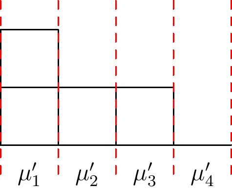
Using Tanisaki’s approach, we can define \[R_{\mu}=\mathbb{C}[x_1,\ldots,x_n]/I_{\mu},\] where $I_{\mu}$ is the ideal generated by the partial elementary symmetric functions defined as follows. Recall that the elementary symmetric function $e_d(z_1,\ldots,z_k)$ is the sum of all square-free monomials of degree $d$ in the set of variables $z_i$. Let $S\subset\{x_1,\ldots,x_n\}$ with $|S|=k$. Then the elementary symmetric function $e_r(S)$ in this subset of the variables is called a partial elementary symmetric function, and we have \[I_{\mu}=(e_r(S) : k-d_k(\mu) \lt r \le k, |S|=k).\] Here, $d_k(\mu)=\mu’_n+\mu’_{n-1}+\cdots+ \mu’_{n-k+1}$ is the number of boxes in the last $k$ columns of $\mu$, where we pad the transpose partition $\mu’$ with $0$’s so that it has $n$ parts.
This ring $R_\mu$ inherits the natural action of $S_n$ on $\mathbb{C}[x_1,\ldots,x_n]$ by permuting the variables, since $I_\mu$ is fixed under this action. Since $I_\mu$ is also a homogeneous ideal, $R_\mu$ is a graded $S_n$-module, graded by degree.
To illustrate the construction, suppose $n=4$ and $\mu=(3,1)$. Then to compute $I_{\mu}$, first consider subsets $S$ of $\{x_1,\ldots,x_4\}$ of size $k=1$. We have $d_1(\mu)=0$ since the fourth column of the Young diagram of $\mu$ is empty (see image below), and so in order for $e_r(S)$ to be in $I_\mu$ we must have $1-0\lt r \le 1$, which is impossible. So there are no partial elementary symmetric functions in $1$ variable in $I_\mu$.
For subsets $S$ of size $k=2$, we have $d_2(\mu)=1$ since there is one box among the last two columns (columns $3$ and $4$) of $\mu$, and we must have $2-1\lt r\le 2$. So $r$ can only be $2$, and we have the partial elementary symmetric functions $e_2(S)$ for all subsets $S$ of size $2$. This gives us the six polynomials \[x_1x_2,\hspace{0.3cm} x_1x_3,\hspace{0.3cm} x_1x_4,\hspace{0.3cm} x_2x_3,\hspace{0.3cm} x_2x_4,\hspace{0.3cm} x_3x_4.\]
For subsets $S$ of size $k=3$, we have $d_3(\mu)=2$, and so $3-2 \lt r\le 3$. We therefore have $e_2(S)$ and $e_3(S)$ for each such subset $S$ in $I_\mu$, and this gives us the eight additional polynomials \[x_1x_2+x_1x_3+x_2x_3, \hspace{0.5cm}x_1x_2+x_1x_4+x_2x_4,\] \[x_1x_3+x_1x_4+x_3x_4,\hspace{0.5cm} x_2x_3+x_2x_4+x_3x_4,\] \[x_1x_2x_3, \hspace{0.4cm} x_1x_2x_4, \hspace{0.4cm} x_1x_3x_4,\hspace{0.4cm} x_2x_3x_4\]
Finally, for $S=\{x_1,x_2,x_3,x_4\}$, we have $d_4(\mu)=4$ and so $4-4\lt r\le 4$. Thus all of the full elementary symmetric functions $e_1,\ldots,e_4$ in the four variables are also relations in $I_{\mu}$. All in all we have \[\begin{align*} I_{(3,1)}= &(e_2(x_1,x_2), e_2(x_1,x_3),\ldots, e_2(x_3,x_4), \\ & e_2(x_1,x_2,x_3), \ldots, e_2(x_2,x_3,x_4), \\ & e_3(x_1,x_2,x_3), \ldots, e_3(x_2,x_3,x_4), \\ & e_1(x_1,\ldots,x_4), e_2(x_1,\ldots,x_4), e_3(x_1,\ldots,x_4), e_4(x_1,\ldots,x_4)) \end{align*}\]
As two more examples, it’s clear that $R_{(1^n)}=\mathbb{C}[x_1,\ldots,x_n]/(e_1,\ldots,e_n)$ is the ring of coninvariants under the $S_n$ action, and $R_{(n)}=\mathbb{C}$ is the trivial representation. So $R_\mu$ is a generalization of the coinvariant ring, and in fact the graded Frobenius characteristic of $R_\mu$ is the Hall-Littlewood polynomial $\widetilde{H}_\mu(x;q)$.
Where do these relations come from? The rings $R_\mu$ were originally defined as follows. Let $A$ be a nilpotent $n\times n$ matrix over $\mathbb{C}$. Then $A$ has all $0$ eigenvalues, and so it is conjugate to a matrix in Jordan normal form whose Jordan blocks have all $0$’s on the diagonal. The sizes of the Jordan blocks, written in nonincreasing order form a partition $\mu’$, and this partition uniquely determines the conjugacy class of $A$. In other words:
There is exactly one nilpotent conjugacy class $C_{\mu’}$ in the space of $n\times n$ matrices for each partition $\mu’$ of $n$.
The closures of these conjugacy classes $\overline{C_{\mu’}}$ form closed matrix varieties, and their coordinate rings were studied here. However, they are easier to get a handle on after intersecting with the set $T$ of diagonal matrices, leading to an interesting natural question: what is the subvariety of diagonal matrices in the closure of the nilpotent conjugacy class $C_{\mu’}$? Defining $R_\mu=\mathcal{O}(\overline{C_{\mu’}}\cap T)$, we obtain the same modules as above.
Tanisaki found the presentation for $R_\mu$ given above using roughly the following argument. Consider the matrix $A-tI$, where $A\in C_{\mu’}$. Then one can show (see, for instance, the discussion of invariant factors and elementary divisors in the article on Smith normal form on Wikipedia) that the largest power of $t$ dividing all of the $k\times k$ minors of $A-tI$, say $t^{d_k}$, is fixed under conjugation, so we can assume $A$ is in Jordan normal form. Then it’s not hard to see, by analyzing the Jordan blocks, that this power of $t$ is $t^{d_k(\mu)}$ where $\mu$ is the transpose partition of $\mu’$ and $d_k(\mu)$ is defined as above - the sums of the ending columns of $\mu$.
It follows that any element of the closure of $C_\mu$ must also have this property, and so if $X=\mathrm{diag}(x_1,\ldots,x_n)\in \overline{C_\mu}\cap T$ then we have \[t^{d_k(\mu)} | (x_{i_1}-t)(x_{i_2}-t)\cdots (x_{i_k}-t)\] for any subset $S=\{x_{i_1},\ldots,x_{i_k}\}$ of $\{x_1,\ldots,x_n\}$. Expanding the right hand side as a polynomial in $t$ using Vieta’s formulas, we see that the elementary symmetric functions $e_r(S)$ vanish on $X$ as soon as $r \gt k-d_k(\mu)$, which is exactly the relations that describe $I_\mu$ above.
It takes somewhat more work to prove that these relations generate the entire ideal, but this can be shown by showing that $R_\mu$ has the right dimension, namely the multinomial coefficient $\binom{n}{\mu}$. And for that, we’ll discuss on page 2 the monomial basis of Garsia and Procesi.
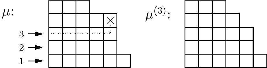
Garsia and Procesi defined the sets of monomials $\mathcal{B}_\mu$ recursively by:
\[\mathcal{B}_{(1)}=\{1\},\] \[\mathcal{B}_{\mu}=\bigcup_d x_n^{d-1} \mathcal{B}_{\mu^{(d)}}\] where $n=|\mu|$ and $\mu^{(d)}$ is the smaller partition formed by removing the corner square that is in column $\mu_d$. They also showed that $\mathcal{B}_\mu$ forms a basis of $R_\mu$ for each $\mu$.
This set can also be described explicitly (see my thesis) in terms of Yamanouchi words. A word $w$ with $\mu_i$ copies of $i-1$ for each $i$ is said to be Yamanouchi if every suffix of the word also has partition content: that is, every tail $w_k,\ldots,w_n$ has at least as many $i-1$’s as $i$’s for each $i$. For instance, $1020010$ is Yamanouchi, but $0100120$ is not because the suffix $20$ has more $2$’s than $1$’s. The partition $\mu$ is called the content of the word; as an example, the word $1020010$ has content $(4,2,1)$ since there are four $0$’s, two $1$’s, and one $2$ in the word. Let $\mathrm{Yam}(\mu)$ be the set of all Yamanouchi words of content $\mu$.
For a word $w$, define $x^w=x_n^{w_1}\cdots x_1^{w_n}$. Then \[\mathcal{B}_\mu=\{x^d:\exists w\in \mathrm{Yam}(\mu), x^d|x^w\}\] is the set of monomials that divide some monomial of a Yamanouchi word of content $\mu$.
The fascinating thing is that this lower order ideal of monomials has size $\binom{n}{\mu}$. This is not immediately obvious, especially since some of the monomials divide more than one Yamanouchi monomial. But one nice way of counting them is by interpreting the degrees of these monomials as generalized Carlitz codes, and tying them to the Macdonald $\mathrm{inv}$ statistic.
First, note that in the case $\mu=(1^n)$, the only Yamanouchi word $w$ of content $\mu$ is $n-1,n-2,\ldots,3,2,1,0$, and so the monomials that divide $x^w$ are precisely those whose degrees form a Carlitz code, as described in this post.
Indeed, consider the Macdonald fillings with distinct entries $1,\ldots, n$ of the transpose $\mu’$ with $\mathrm{maj}(\sigma)=0$, as described in this post (we will be using all the notation from that post from here on). This condition means that all the columns are weakly increasing when read from top to bottom, and there are no other restrictions on the filling. The $\mathrm{inv}$ statistic on such tableaux can be computed by counting the number of attacking pairs, since there are no descents. If we assign to an entry $i$ the number $a(i)$ of attacking pairs that involve $i$ as the smaller entry, then it turns out that the resulting monomials $\prod x_{n-i}^{a(i)}$ are exactly the monomials of $\mathcal{B}_\mu$.
Since there are exactly $\binom{n}{\mu}$ ways to choose which entries go in each column of our filling, and only one way to make the columns increasing once we made that choice, it’s an immediate consequence that $\|\mathcal{B}_\mu\|=\binom{n}{\mu}$.