What do Schubert curves, Young tableaux, and K-theory have in common? (Part III)

This is the third and final post in our expository series of posts (see Part I and Part II) on the recent paper coauthored by Jake Levinson and myself.

Last time, we discussed the fact that the operator $\omega$ on certain Young tableaux is actually the monodromy operator of a certain covering map from the real locus of the Schubert curve $S$ to $\mathbb{RP}^1$. Now, we’ll show how our improved algorithm for computing $\omega$ can be used to approach some natural questions about the geometry of the curve $S$. For instance, how many (complex) connected components does $S$ have? What is its genus? Is $S$ a smooth (complex) curve?

The genus of $S$

The arithmetic genus of a connected curve $S$ can be defined as $g=1-\chi(\mathcal{O}_S)$ where \[\chi(\mathcal{O}_S)=\dim H^0(\mathcal{O}_S)-\dim H^1(\mathcal{O}_S)\] is the Euler characteristic and $\mathcal{O}_S$ is the structure sheaf. So, to compute the genus it suffices to compute the Euler characteristic, which can alternatively be defined in terms of the $K$-theory of the Grassmannian.

The $K$-theory ring $K(\mathrm{Gr}(n,k))$

The $K$-theory ring $K(X)$ of a scheme $X$ is defined as follows. First, consider the free abelian group $G$ generated by isomorphism classes of locally free coherent sheaves (a.k.a. vector bundles) on $X$. Then define $K(X)$, as a group, to be the quotient of $G$ by ``short exact sequences’’, that is, the quotient $G/H$ where $H$ is the subgroup generated by expressions of the form $[\mathcal{E}_1]+[\mathcal{E}_2]-[\mathcal{E}]$ where $0\to \mathcal{E}_1 \to \mathcal{E} \to \mathcal{E}_2 \to 0$ is a short exact sequence of vector bundles on $X$. This gives the additive structure on $K(X)$, and the tensor product operation on vector bundles makes it into a ring. It turns out that, in the case that $X$ is smooth (such as a Grassmannian!) then we get the exact same ring if we remove the ``locally free’’ restriction and consider coherent sheaves modulo short exact sequences.

Where does this construction come from? Well, a simpler example of $K$-theory is the construction of the Grothendieck group of an abelian monoid. Consider an abelian monoid M (recall that a monoid is a set with an associative binary operation and an identity element, like a group without inverses). We can construct an associated group $K(M)$ by taking the quotient free abelian group generated by elements $[m]$ for $m\in M$ by the subgroup generated by expressions of the form $[m]+[n]-[m+n]$. So, for instance, $K(\mathbb{N})=\mathbb{Z}$. In a sense we are groupifying monoids. The natural monoidal operation on vector spaces is $\oplus$, so if $X$ is a point, then all short exact sequences split and the $K$-theory ring $K(X)$ is the Grothendieck ring of this monoid.

A good exposition on the basics of $K$-theory can be found here, and for the $K$-theory of Grassmannians, see Buch’s paper. For now, we’ll just give a brief description of how the $K$-theory of the Grassmannian works, and how it gives us a handle on the Euler characteristic of Schubert curves.

Recall from this post that the CW complex structure given by the Schubert varieties shows that the classes $[\Omega_\lambda]$, where $\lambda$ is a partition fitting inside a $k\times (n-k)$ rectangle, generate the cohomology ring $H^\ast(\mathrm{Gr}(n,k))$. Similarly, the $K$-theory ring is a filtered ring generated by the classes of the coherent sheaves $[\mathcal{O}_{\lambda}]$ where if $\iota$ is the inclusion map $\iota:\Omega_\lambda\to \mathrm{Gr}(n,k)$, then $\mathcal{O}_\lambda=\iota_\ast \mathcal{O}_{\Omega_\lambda}$. Multiplication of these basic classes is given by a variant of the Littlewood-Richardson rule: \[[\mathcal{O}_\lambda]\cdot [\mathcal{O}_\nu]=\sum_\nu (-1)^{|\nu|-|\lambda|-|\mu|}c^\nu_{\lambda\mu}[\mathcal{O}_\nu]\] where if $|\nu|=|\lambda|+|\mu|$ then $c^{\nu}_{\lambda\mu}$ is the usual Littlewood-Richardson coefficient. If $|\nu|<|\lambda|+|\mu|$ then the coefficient is zero, and if it $|\nu|>|\lambda|+|\mu|$ then $c^{\nu}_{\lambda\mu}$ is a nonnegative integer. We will refer to these nonnegative values as $K$-theory coefficients.

$K$-theory and the Euler characteristic

The $K$-theory ring is especially useful in computing Euler characteristics. It turns out that the Euler characteristic gives an (additive) group homomorphism $\chi:K(X)\to \mathbb{Z}$. To show this, it suffices to show that if $0\to \mathcal{A}\to \mathcal{B}\to \mathcal{C}\to 0$ is a short exact sequence of coherent sheaves on $X$, then $\chi(\mathcal{A})+\chi(\mathcal{C})-\chi(\mathcal{B})=0$. Indeed, such a short exact sequence gives rise to a long exact sequence in cohomology:

\[ \begin{array}{cccccc} & H^0(\mathcal{A}) & \to & H^0(\mathcal{B}) & \to & H^0(\mathcal{C}) \\ \to &H^1(\mathcal{A}) & \to & H^1(\mathcal{B}) & \to & H^1(\mathcal{C}) \\ \to &H^2(\mathcal{A}) & \to & H^2(\mathcal{B}) & \to & H^2(\mathcal{C}) \\ \cdots & & & & & \end{array} \]

and the alternating sum of the dimensions of any exact sequence must be zero. Thus we have \[\begin{eqnarray*}0&=&\sum_i (-1)^i\dim H^i(\mathcal{A})-\sum_i (-1)^i\dim H^i(\mathcal{b})+\sum_i (-1)^i\dim H^i(\mathcal{C}) \\ &=&\chi(\mathcal{A})+\chi(\mathcal{C})-\chi(\mathcal{B})\end{eqnarray*}\] as desired.

Therefore, it makes sense to talk about the Euler characteristic of a class of coherent sheaves in $K(X)$. In fact, in our situation, we have a closed subset $S$ of $X=\mathrm{Gr}(n,k)$, say with inclusion map $j:S\to X$, and so the Euler characteristic of the pushforward $j_\ast\mathcal{O}_S$ is equal to $\chi(\mathcal{O}_S)$ itself. We can now compute the Euler characteristic $\chi(j_\ast\mathcal{O}_S)$ using the structure of the $K$-theory ring of the Grassmannian. Indeed, $S$ is the intersection of Schubert varieties indexed by the three partitions $\alpha$, $\beta$, and $\gamma$ (see Part I). So in the $K$-theory ring, if we identify structure sheaves of closed subvarieties with their pushforwards under inclusion maps, we have \[[\mathcal{O}_S]=[\mathcal{O}_\alpha]\cdot [\mathcal{O}_\beta]\cdot [\mathcal{O}_\gamma].\] By the $K$-theoretic Littlewood-Richardson rule described above, this product expands as a sum of integer multiples of classes $[\mathcal{O}_\nu]$ where $|\nu|\ge |\alpha|+|\beta|+|\gamma|$. But in our setup we have $|\alpha|+|\beta|+|\gamma|=k(n-k)-1$, so $\nu$ is either the entire $k\times (n-k)$ rectangle (call this $\rho$) or it is the rectangle minus a single box (call this $\rho’$). In other words, we have:

\[[\mathcal{O}_S]=c^{\rho’}_{\alpha,\beta,\gamma}[\mathcal{O}_{\rho’}]-k[\mathcal{O}_{\rho}]\] where $k$ is an integer determined by the $K$-theory coefficients. Notice that $c^{\rho’}_{\alpha,\beta,\gamma}$ is the usual Littlewood-Richardson coefficient, and counts exactly the size of the fibers (the set $\omega$ acts on) in our map from Part II. Let’s call this number $N$.

Finally, notice that $\Omega_\rho$ and $\Omega_{\rho’}$ are a point and a copy of $\mathbb{P}^1$ respectively, and so both have Euler characteristic $1$. It follows that \[\chi(\mathcal{O}_S)=N-k.\] Going back to the genus, we see that if $S$ is connected, we have $g=1-\chi(\mathcal{O}_S)=k-(N-1)$.

Computing $k$ in terms of $\omega$

The fascinating thing about our algorithm for $\omega$ is that certain steps of the algorithm combinatorially correspond to certain tableaux that enumerate the $K$-theory coefficients, giving us information about the genus of $S$. These tableaux are called ``genomic tableaux’’, and were first introduced by Pechenik and Yong.

In our case, the genomic tableaux that enumerate $k$ can be defined as follows. The data of a tableau $T$ and two marked squares $\square_1$ and $\square_2$ in $T$ is a genomic tableau if:

The marked squares are non-adjacent and contain the same entry $i$,
There are no $i$’s between $\square_1$ and $\square_2$ in the reading word of $T$,
If we delete either $\square_1$ or $\square_2$, every suffix of the resulting reading word is ballot (has more $j$’s than $j+1$’s for all $j$).

For instance, consider the following tableaux with two marked (shaded) squares:

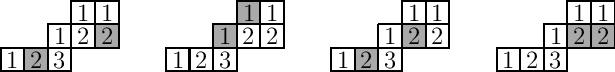
Property 1 means that the fourth tableau is not genomic: the marked squares, while they do contain the same entry, are adjacent squares. The first tableau above violates Property 2, because there is a $2$ between the two marked $2$’s in reading order. Finally, the second tableau above violates Property 3, because if we delete the top marked $1$ then the suffix $221$ is not ballot. The third tableau above satisfies all three properties, and so it is genomic.

Finally, consider the algorithm for $\omega$ described in Part I. Jake and I discovered that the steps in Phase 1 in which the special box does not move to an adjacent square are in bijective correspondence with the $K$-theory tableau of the total skew shape $\gamma^c/\alpha$ and content $\beta$ (where the marked squares only add $1$ to the total number of $i$’s). The correspondence is formed by simply filling the starting and ending positions of the special box with the entry $i$ that it moved past, and making these the marked squares of a genomic tableau. In other words:

The $K$-theory coefficient $k$ is equal to the number of non-adjacent moves in all Phase 1’s of the local algorithm for $\omega$.

Geometric consequences

This connection allows us to get a handle on the geometry of the Schubert curves $S$ using our new algorithm. As one illuminating example, let’s consider the case when $\omega$ is the identity permutation.

It turns out that the only way for $\omega$ to map a tableau back to itself is if Phase 1 consists of all vertical slides and Phase 2 is all horizontal slides; then the final shuffle step simply reverses these moves. This means that we have no non-adjacent moves, and so $k=0$ in this case. Since $\omega$, the monodromy operator on the real locus, is the identity, we also know that the number of real connected components is equal to $N$, which is an upper bound on the number of complex connected components (see here), which in turn is an upper bound on the Euler characteristic $\chi(\mathcal{O}_S)=\dim H^0(\mathcal{O}_S)-\dim H^1(\mathcal{O}_S)$. But the Euler characteristic is equal to $N$ in this case, and so there must be $N$ complex connected components, one for each of the real connected components. It follows that $\dim H^1(\mathcal{O}_S)=0$, so the arithmetic genus of each of these components is zero.

We also know each of these components is integral, and so they must each be isomorphic to $\mathbb{CP}^1$ (see Hartshorne, section 4.1 exercise 1.8). We have therefore determined the entire structure of the complex Schubert curve $S$ in the case that $\omega$ is the identity map, using the connection with $K$-theory described above.

Similar analyses lead to other geometric results: we have also shown that the Schubert curves $S$ can have arbitrarily high genus, and can arbitrarily many complex connected components, for various values of $\alpha$, $\beta$, and $\gamma$.

So, what do Schubert curves, Young tableaux, and $K$-theory have in common? A little monodromy operator called $\omega$.