What do Schubert curves, Young tableaux, and K-theory have in common? (Part II)

In the last post, we discussed an operation $\newcommand{\box}{\square} \omega$ on skew Littlewood-Richardson Young tableaux with one marked inner corner, defined as a commutator of rectification and shuffling. As a continuation, we’ll now discuss where this operator arises in geometry.

Schubert curves: Relaxing a Restriction

Recall from our post on Schubert calculus that we can use Schubert varieties to answer the question:

Given four lines $\ell_1,\ell_2,\ell_3,\ell_4\in \mathbb{C}\mathbb{P}^3$, how many lines intersect all four of these lines in a point?

In particular, given a complete flag, i.e. a chain of subspaces \[0=F_0\subset F_1\subset\cdots \subset F_m=\mathbb{C}^m\] where each $F_i$ has dimension $i$, the Schubert variety of a partition $\lambda$ with respect to this flag is a subvariety of the Grassmannian $\mathrm{Gr}^n(\mathbb{C}^m)$ defined as \[\Omega_{\lambda}(F_\bullet)=\{V\in \mathrm{Gr}^n(\mathbb{C}^m)\mid \dim V\cap F_{n+i-\lambda_i}\ge i.\}\]

Here $\lambda$ must fit in a $k\times (n-k)$ box in order for the Schubert variety to be nonempty. In the case of the question above, we can translate the question into an intersection problem in $\mathrm{Gr}^2(\mathbb{C}^4)$ with four general two-dimensional subspaces $P_1,P_2,P_3,P_4\subset \mathbb{C}^4$, and construct complete flags $F_\bullet^{(1)},F_\bullet^{(2)},F_\bullet^{(3)},F_\bullet^{(4)}$ such that their second subspace $F^{(i)}_2$ is $P_i$ for each $i=1,2,3,4$. Then the intersection condition is the problem of finding a plane that intersects all $P_i$’s in a line. The variety of all planes intersecting $P_i$ in a line is $\Omega_\box(F_\bullet^{(i)})$ for each $i$, and so the set of all solutions is the intersection \[\Omega_\box(F_\bullet^{(1)})\cap \Omega_\box(F_\bullet^{(2)})\cap \Omega_\box(F_\bullet^{(3)})\cap \Omega_\box(F_\bullet^{(4)}).\] And, as discussed in our post on Schubert calculus, since the $k\times(n-k)$ box has size $4$ in $\mathrm{Gr}^2(\mathbb{C}^4)$ and the four partitions involved have sizes summing to $4$, this intersection has dimension $0$. The Littlewood-Richardson rule then tells us that the number of points in this zero-dimensional intersection is the Littlewood-Richardson coefficient $c_{\box,\box,\box,\box}^{(2,2)}$.

What happens if we relax one of the conditions in the problem, so that we are only intersecting three of the Schubert varieties above? In this case we get a one-parameter family of solutions, which we call a Schubert curve.

To define a Schubert curve in general, we require a sufficiently ``generic’’ choice of $r$ flags $F_\bullet^{(1)},\ldots, F_\bullet^{(r)}$ and a list of $r$ partitions $\lambda^{(1)},\ldots,\lambda^{(r)}$ (fitting inside the $k\times (n-k)$ box) whose sizes sum to $k(n-k)-1$. It turns out that one can choose any flags $F_\bullet$ defined by the iterated derivatives at chosen points on the rational normal curve, defined by the locus of points of the form \[(1:t:t^2:t^3:\cdots:t^{n-1})\in \mathbb{CP}^n\] (along with the limiting point $(0:0:\cdots:1)$.) In particular, consider the flag whose $k$th subspace $F_k$ is the span of the first $k$ rows of the matrix of iterated derivatives at the point on this curve parameterized by $t$: \[\left(\begin{array}{cccccc} 1 & t & t^2 & t^3 & \cdots & t^{n-1} \\ 0 & 1 & 2t & 3t^2 & \cdots & (n-1) t^{n-2} \\ 0 & 0 & 2 & 6t & \cdots & \frac{(n-1)!}{(n-3)!} t^{n-3} \\ 0 & 0 & 0 & 6 & \cdots & \frac{(n-1)!}{(n-4)!} t^{n-3} \\ \vdots & \vdots & \vdots & \vdots &\ddots & \vdots \\ 0 & 0 & 0 & 0 & \cdots & (n-1)! \end{array}\right)\]

This is called the osculating flag at the point $t$, and if we pick a number of points on the curve and choose their osculating flag, it turns out that they are in sufficiently general position in order for the Schubert intersections to have the expected dimension. So, we pick some number $r$ of these osculating flags, and choose exactly $r$ partitions $\lambda^{(1)},\ldots,\lambda^{(r)}$ with sizes summing to $k(n-k)-1$. Intersecting the resulting Schubert varieties defines a Schubert curve $S$.

A covering map

In order to get a handle on these curves, we consider the intersection of $S$ with another Schubert variety of a single box, $\Omega_\box(F_\bullet)$. In particular, after choosing our $r$ osculating flags, choose an $(r+1)$st point $t$ on the rational normal curve and choose the single-box partition $\lambda=(1)$. Intersecting the resulting Schubert variety $\Omega_\box(F_\bullet)$ with our Schubert curve $S$ gives us a zero-dimensional intersection, with the number of points given by the Littlewood-Richardson coefficient $c:=c^{B}_{\lambda^{(1)},\ldots,\lambda^{(r)},\box}$ where $B=((n-k)^k)$ is the $k\times (n-k)$ box partition.

By varying the choice of $t$, we obtain a partition of an open subset of the Schubert curve into sets of $c$ points. We can then define a map from this open subset of $S$ to the points of $\mathbb{CP}^1$ for which the preimage of $(1:t)$ consists of the $c$ points in the intersection given by choosing the $(r+1)$st point to be $(1:t:t^2:t^3:\cdots:t^{n-1})$.

In this paper written by my coauthor Jake Levinson, it is shown that if we choose all $r+1$ points to be real, then this can be extended to a map $S\to \mathbb{CP}^1$ for which the real locus $S(\mathbb{R})$ is a smooth, finite covering of $\mathbb{RP}^1$. The fibers of this map have size $c=c^{B}_{\lambda^{(1)},\ldots,\lambda^{(r)},\box}$. Note that this Littlewood-Richardson coefficient counts the number of ways of filling the box $B$ with skew Littlewood-Richardson tableaux with contents $\lambda^{(1)},\ldots,\lambda^{(r)},\box$ such that each skew shape extends the previous shape outwards. In addition, by the symmetry of Littlewood-Richardson coefficients, it doesn’t matter what order in which we use the partitions. It turns out that there is a canonical way of labeling the fibers by these chains of tableaux, for which the monodromy of the covering is described by shuffling operators.

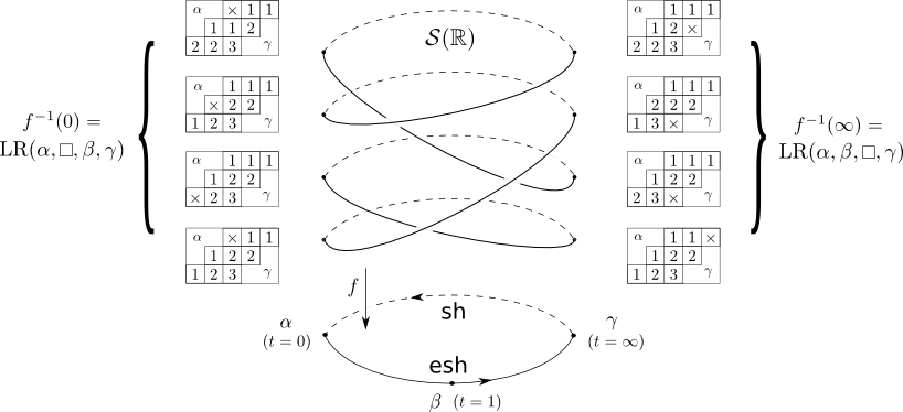
Let’s be more precise, and consider the simplest interesting case, $r=3$. We have three partitions $\alpha$, $\beta$, and $\gamma$ such that \[|\alpha|+|\beta|+|\gamma|=k(n-k)-1=|B|-1.\] Let’s choose, for simplicity, the three points $0$, $1$, and $\infty$ to define the respective osculating flags. Then we can label the points in the fiber $f^{-1}(0)$ of the map $f:S\to \mathbb{RP}^1$ by the fillings of the box with a chain of Littlewood-Richardson tableaux of contents $\alpha$, $\box$, $\beta$, and $\gamma$ in that order. Note that there is only one Littlewood-Richardson tableau of straight shape and content $\alpha$, and similarly for the anti-straight shape $\gamma$, so the data here consists of a skew Littlewood-Richardson tableau of content $\beta$ with an inner corner chosen to be the marked box. This is the same object that we were considering in Part I.

Now, we can also label the fiber $f^{-1}(1)$ by the chains of contents $\box$, $\alpha$, $\beta$, and $\gamma$ in that order, and finally label the fiber $f^{-1}(\infty)$ by the chains of contents $\alpha$, $\beta$, $\box$, and $\gamma$ in that order, in such a way that if we follow the curve $S$ along an arc from a point in $f^{-1}(0)$ to $f^{-1}(1)$ or similarly from $1$ to $\infty$ or $\infty$ to $0$, then then the map between the fibers is given by the shuffling operations described in the last post! In particular if we follow the arc from $0$ to $\infty$ that passes through $1$, the corresponding operation on the fibers is given by the ``evacuation-shuffle’’, or the first three steps of the operator $\omega$ described in the previous post. The arc from $\infty$ back to $0$ on the other side is given by the ``shuffle’’ of the $\box$ past $\beta$, which is the last step of $\omega$. All in all, $\omega$ gives us the monodromy operator on the zero fiber $f^{-1}(0)$.

The following picture sums this up:

So, the real geometry of the Schubert curve boils down to an understanding of the permutation $\omega$. Our local algorithm allows us to get a better handle on the orbits of $\omega$, and hence tell us things about the number of real connected components, the lengths of these orbits, and even in some cases the geometry of the complex curve $S$.

Next time, I’ll discuss some of these consequences, as well as some fascinating connections to the $K$-theory of the Grassmannian. Stay tuned!