What do Schubert curves, Young tableaux, and K-theory have in common? (Part I)

In a recent and fantastic collaboration between Jake Levinson and myself, we discovered new links between several different geometric and combinatorial constructions. We’ve weaved them together into a beautiful mathematical story, a story filled with drama and intrigue.

So let’s start in the middle.

Slider puzzles for mathematicians

Those of you who played with little puzzle toys growing up may remember the “15 puzzle”, a $4\times 4$ grid of squares with 15 physical squares and one square missing. A move consisted of sliding a square into the empty square. The French name for this game is “jeu de taquin”, which translates to “the teasing game”.

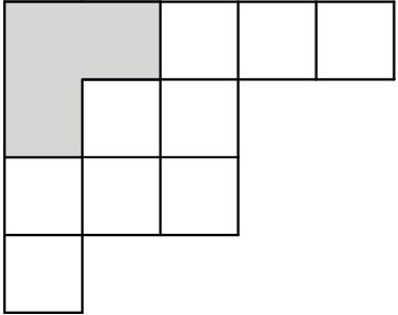
We can play a similar jeu de taquin game with semistandard Young tableaux. To set up the board, we need a slightly more general definition: a skew shape $\lambda/\mu$ is a diagram of squares formed by subtracting the Young diagram (see this post) of a partition $\mu$ from the (strictly larger) Young diagram of a partition $\lambda$. For instance, if $\lambda=(5,3,3,1)$ and $\mu=(2,1)$, then the skew shape $\lambda/\mu$ consists of the white squares shown below.

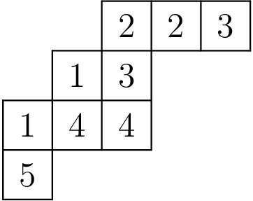
A semistandard Young tableau is then a way of filling the squares in such a skew shape with positive integers in such a way that the entries are weakly increasing across rows and strictly increasing down columns:

Now, an inner jeu de taquin slide consists of choosing an empty square adjacent to two of the numbers, and successively sliding entries inward into the empty square in such a way that the tableau remains semistandard at each step. This is an important rule, and it implies that, once we choose our inner corner, there is a unique choice between the squares east and south of the empty square at each step; only one can be slid to preserve the semistandard property. An example of an inwards jeu de taquin slide is shown (on repeat) in the animation below:

Here’s the game: perform a sequence of successive jeu de taquin slides until there are no empty inner corners left. What tableaux can you end up with? It turns out that, in fact, it doesn’t matter how you play this game! No matter which inner corner you pick to start the jeu de taquin slide at each step, you will end up with the same tableau in the end, called the rectification of the original tableau.

Since we always end up at the same result, it is sometimes more interesting to ask the question in reverse: can we categorize all skew tableaux that rectify to a given fixed tableau? This question has a nice answer in the case that we fix the rectification to be superstandard, that is, the tableau whose $i$th row is filled with all $i$’s:

It turns out that a semistandard tableau rectifies to a superstandard tableau if and only if it is Littlewood-Richardson, defined as follows. Read the rows from bottom to top, and left to right within a row, to form the reading word. Then the tableau is Littlewood-Richardson if every suffix (i.e. consecutive subword that reaches the end) of the reading word is ballot, which means that it has at least as many $i$’s as $i+1$’s for each $i\ge 1$.

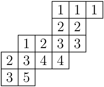
For instance, the Littlewood-Richardson tableau below has reading word 352344123322111, and the suffix 123322111, for instance, has at least as many $1$’s as $2$’s, $2$’s as $3$’s, etc. Littlewood-Richardson tableaux are key to the Littlewood-Richardson rule, which allows us to efficiently compute products of Schur functions.

A convoluted commutator

The operation that Jake and I studied is a sort of commutator of rectification with another operation called ``shuffling’’. The process is as follows. Start with a Littlewood-Richardson tableau $T$, with one of the corners adjacent to $T$ on the inside marked with an ``$\times$’’. Call this extra square the ``special box’’. Then we define $\omega(T)$ to be the result of the following four operations applied to $T$.

1. Rectification: Treat $\times$ as having value $0$ and rectify the entire skew tableau.
2. Shuffling: Treat the $\times$ as the empty square to perform an inward jeu de taquin slide. The resulting empty square on the outer corner is the new location of $\times$.
3. Un-rectification: Treat $\times$ as having value $\infty$ and un-rectify, using the sequence of moves from the rectification step in reverse.
4. Shuffling back: Treat the $\times$ as the empty square to perform a reverse jeu de taquin slide, to move the $\times$ back to an inner corner.

We can iterate $\omega$ to get a permutation on all pairs $(\times,T)$ of a Littlewood-Richardson tableau $T$ with a special box marked on a chosen inner corner, with total shape $\lambda/\mu$ for some fixed $\lambda$ and $\mu$. As we’ll discuss in the next post, this permutation is related to the monodromy of a certain covering space of $\mathbb{RP}^1$ arising from the study of Schubert curves. But I digress.

One of the main results in our paper provides a new, more efficient algorithm for computing $\omega(T)$. In particular, the first three steps of the algorithm are what we call the ``evacuation-shuffle’’, and our local rule for evacuation shuffling is as follows:

1. Phase 1. If the special box does not precede all of the $i$’s in reading order, switch the special box with the nearest $i$ prior to it in reading order. Then increment $i$ by $1$ and repeat this step.

   If, instead, the special box precedes all of the $i$’s in reading order, go to Phase 2.

2. Phase 2. If the suffix of the reading word starting at the special box has more $i$’s than $i+1$’s, switch the special box with the nearest $i$ after it in reading order whose suffix has the same number of $i$’s as $i+1$’s. Either way, increment $i$ by $1$ and repeat this step until $i$ is larger than any entry of $T$.

So, to get $\omega(T)$, we first follow the Phase 1 and Phase 2 steps, and then we slide the special box back with a simple jeu de taquin slide. We can then iterate $\omega$, and compute an entire $\omega$-orbit, a cycle of its permutation. An example of this is shown below.

That’s all for now! In the next post I’ll discuss the beginning of the story: where this operator $\omega$ arises in geometry and why this algorithm is exactly what we need to understand it.