Schubert Calculus
I recently gave a talk on Schubert calculus in the Student Algebraic Geometry Seminar at UC Berkeley. As a combinatorialist, this is a branch of enumerative geometry that particularly strikes my fancy. I also made a handout for the talk called ``Combinatorics for Algebraic Geometers,’’ and I thought I’d post it here in blog format.
Motivation
Enumerative geometry
In the late 1800’s, Hermann Schubert investigated problems in what is now called enumerative geometry, or more specifically, Schubert calculus. As some examples, where all projective spaces are assumed to be over the complex numbers:
- How many lines in $\mathbb{P}^n$ pass through two given points? Answer: One, as long as the points are distinct.3. How many planes in $\mathbb{P}^3$ contain a given line $l$ and a given point $P$? Answer: One, as long as $P\not\in l$.5. How many lines in $\mathbb{P}^3$ intersect four given lines $l_1,l_2,l_3,l_4$? Answer: Two, as long as the lines are in sufficiently ``general” position.7. How many $(r-1)$-dimensional subspaces of $\mathbb{P}^{m-1}$ intersect each of $r\cdot (m-r)$ general subspaces of dimension $m-r-1$ nontrivially? Answer: \[\frac{(r(m-r))!\cdot (r-1)!\cdot (r-2)!\cdot \cdots\cdot 1!}{(m-1)!\cdot(m-2)!\cdot\cdots\cdot 1!}\]
The first two questions are not hard, but how would we figure out the other two? And what do we mean by ``sufficiently general position’’?
Schubert’s 19th century solution to problem 3 above would have invoked what he called the ``Principle of Conservation of Number,” as follows. Suppose the four lines were arranged so that $l_1$ and $l_2$ intersect at a point $P$, $l_3$ and $l_4$ intersect at $Q$, and none of the other pairs of lines intersect. Then the planes formed by each pair of crossing lines intersect at another line $\alpha$, which necessarily intersects all four lines. The line $\beta$ through $P$ and $Q$ also intersects all four lines, and it is not hard to see that these are the only two in this case.
Schubert would have said that since there are two solutions in this configuration and it is a finite number of solutions, it is true for every configuration of lines for which the number is finite by continuity. Unfortunately, due to degenerate cases involving counting with multiplicity, this led to many errors in computations in harder questions of enumerative geometry. Hilbert’s 15th problem asked to put Schubert’s enumerative methods on a rigorous foundation. This led to the modern-day theory known as Schubert calculus.
Describing moduli spaces
Schubert calculus can also be used to describe intersection properties in simpler ways. As we will see, it will allow us to easily prove statements such as:
The variety of all lines in $\mathbb{P}^4$ that are both contained in a general $3$-dimensional hyperplane $S$ and intersect a general line $l$ nontrivially is isomorphic to the variety of all lines in $S$ passing through a specific point in that hyperplane.
(Here, the specific point in the hyperplane is the intersection of $S$ and $L$.)
The Grassmannian
The first thing we need to do to simplify our life is to get out of projective space. Recall that $\mathbb{P}^m$ can be defined as the collection of lines through the origin in $\mathbb{C}^{m+1}$. Furthermore, lines in $\mathbb{P}^m$ correspond to planes through the origin in $\mathbb{C}^{m+1}$, and so on.
In problem $3$ in the introduction, we are trying to find lines in $\mathbb{P}^3$ with certain intersection properties. This translates to a problem about planes through the origin in $\mathbb{C}^4$, which we refer simply as $2$-dimensional subspaces of $\mathbb{C}^4$. We wish to know which $2$-dimensional subspaces $V$ intersect each of four given $2$-dimensional subspaces $W_1,W_2, W_3, W_4$ in at least a line. Our strategy will be to consider the algebraic varieties $Z_i$, $i=1,\ldots,4$, of all possible $V$ intersecting $W_i$ in at least a line, and find the intersection $Z_1\cap Z_2\cap Z_3\cap Z_4$. Each $Z_i$ is an example of a Schubert variety, a moduli space of subspaces of $\mathbb{C}^m$ with specified intersection properties.
The simplest example of a Schubert variety, where we have no constraints on the subspaces, is the Grassmannian $ \Gr^n(\mathbb{C}^m)$.
The Grassmannian $\Gr^n(\mathbb{C}^m)$ is the collection of codimension-$n$ subspaces of $\mathbb{C}^m$. In what follows we will set \[r=m-n,\] so that the codimension-$n$ subspaces have dimension $r$.
We will see later that the Grassmannian has the structure of an algebraic variety, and has two natural topologies that come in handy. For this reason we will call its elements the points of the $\Gr^n(\mathbb{C}^m)$, even though they’re ``actually’’ subspaces of $\mathbb{C}^m$ of dimension $r=m-n$. It’s the same misfortune that causes us to refer to a line through the origin as a ``point in projective space.’’
Now, every point of the Grassmannian is the span of $r$ independent row vectors of length $m$, which we can arrange in an $r\times m$ matrix. For instance, the following represents a point in $\Gr^3(\mathbb{C}^7)$. \[\left[\begin{array}{ccccccc} 0 & -1 & -3 & -1 & 6 & -4 & 5 \\ 0 & 1 & 3 & 2 & -7 & 6 & -5 \\ 0 & 0 & 0 & 2 & -2 & 4 & -2 \end{array}\right]\] Notice that we can perform elementary row operations on the matrix without changing the point of the Grassmannian it represents. Therefore:
Each point of the Grassmannian corresponds to a unique full-rank matrix in reduced row echelon form.
Let’s use the convention that the pivots will be in order from left to right and bottom to top.
Example. In the matrix above we can switch the second and third rows, and then add the third row to the first to get: \[\left[\begin{array}{ccccccc} 0 & 0 & 0 & 1 & -1 & -2 & 0 \\ 0 & 0 & 0 & 2 & -2 & 4 & -2 \\ 0 & 1 & 3 & 2 & -7 & 6 & -5 \\ \end{array}\right]\] Here, the bottom left $1$ was used as the pivot to clear its column. We can now use the $2$ at the left of the middle row as our new pivot, by dividing that row by $2$ first, and adding or subtracting from the two other rows: \[\left[\begin{array}{ccccccc} 0 & 0 & 0 & 0 & 0 & 0 & 1 \\ 0 & 0 & 0 & 1 & -1 & 2 & -1 \\ 0 & 1 & 3 & 0 & -5 & 2 & -3 \\ \end{array}\right]\] Finally we can use the $1$ in the upper right corner to clear its column: \[\left[\begin{array}{ccccccc} 0 & 0 & 0 & 0 & 0 & 0 & 1 \\ 0 & 0 & 0 & 1 & -1 & 2 & 0 \\ 0 & 1 & 3 & 0 & -5 & 2 & 0 \\ \end{array}\right],\] and we are done.
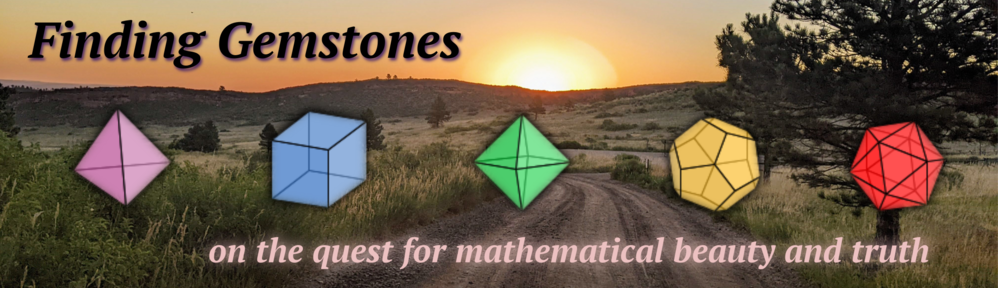
In the preceding example, we were left with a reduced row echelon matrix in the form \[\left[\begin{array}{ccccccc} 0 & 0 & 0 & 0 & 0 & 0 & 1 \\ 0 & 0 & 0 & 1 & \ast & \ast & 0 \\ 0 & 1 & \ast & 0 & \ast & \ast & 0 \\ \end{array}\right],\] i.e. its leftmost $1$’s are in columns $2$, $4$, and $7$. The subset of the Grassmannian whose points have this particular form constitutes a Schubert cell.
Schubert varieties and cell complex structure
To make the previous discussion rigorous, we assign to the matrices of the form \[\left[\begin{array}{ccccccc} 0 & 0 & 0 & 0 & 0 & 0 & 1 \\ 0 & 0 & 0 & 1 & \ast & \ast & 0 \\ 0 & 1 & \ast & 0 & \ast & \ast & 0 \\ \end{array}\right]\] a partition - a nonincreasing sequence of nonnegative integers $\lambda=(\lambda_1,\ldots,\lambda_r)$ - as follows. Cut out the ``upside-down staircase’’ from the left of the matrix, and let $\lambda_i$ be the distance from the end of the staircase to the $1$ in each row. In the matrix above, we get the partition $\lambda=(4,2,1)$. Notice that we always have $\lambda_1\ge \lambda_2\ge \cdots \ge \lambda_r$.
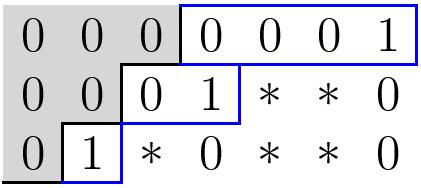
By identifying the partition with its Young diagram, we can alternatively define $\lambda$ as the complement in a $r\times n$ box (recall $n=m-r$) of the diagram $\mu$ defined by the $\ast$’s, where we place the $\ast$’s in the lower right corner. For instance:
Notice that every partition $\lambda$ we obtain in this manner must fit in the $r\times n$ box. For this reason, we will call it the Important Box. (Warning: this terminology is not standard.)
The Schubert cell $\Omega_{\lambda}^\circ\subset \Gr^n(\mathbb{C}^m)$ is the set of points whose row echelon matrix has corresponding partition $\lambda$.
Notice that since each $\ast$ can be filled with any complex number, we have $\Omega_{\lambda}^{\circ}\cong \mathbb{C}^{r\cdot n-\|\lambda \|}$. Thus we can think of the Schubert cells as forming an open cover of the Grassmannian by affine subsets.
More rigorously, the Grassmannian can be viewed as a projective variety by embedding $\Gr^n(\mathbb{C}^m)$ in $\mathbb{P}^{\binom{m}{r}-1}$ via the Plücker embedding. To do so, order the $r$-element subsets $S$ of $\{1,2,\ldots,m\}$ arbitrarily and use this ordering to label the homogeneous coordinates $x_S$ of $\mathbb{P}^{\binom{m}{r}-1}$. Now, given a point in the Grassmannian represented by a matrix $M$, let $x_S$ be the determinant of the $r\times r$ submatrix determined by the columns in the subset $S$. This determines a point in projective space since row operations can only change the coordinates up to a constant factor, and the coordinates cannot all be zero since the matrix has rank $r$.
One can show that the image is an algebraic subvariety of $\mathbb{P}^{\binom{m}{r}-1}$, cut out by homogeneous quadratic relations known as the Plücker relations. (See Miller and Sturmfels, chapter 14.) The Schubert cells form an open affine cover.
We are now in a position to define the Schubert varieties as closed subvarieties of the Grassmannian.
The standard Schubert variety corresponding to a partition $\lambda$, denoted $\Omega_\lambda$, is the closure $\overline{ {\Omega_\lambda}^\circ}$ of the corresponding Schubert cell in the Grassmannian, taken with respect to the Zariski topology. Explicitly, \[\Omega_{\lambda}=\{V\in \mathrm{Gr}^n(\mathbb{C}^m)\mid \dim V\cap \langle e_1,\ldots, e_{n+i-\lambda_i}\rangle \ge i.\}\]
In general, however, we can use a different basis than the standard basis $e_1,\cdots,e_m$ for $\mathbb{C}^m$. Given a complete flag, i.e. a chain of subspaces \[0=F_0\subset F_1\subset\cdots \subset F_m=\mathbb{C}^m\] where each $F_i$ has dimension $i$, we can define \[\Omega_{\lambda}(F_\bullet)=\{V\in \mathrm{Gr}^n(\mathbb{C}^m)\mid \dim V\cap F_{n+i-\lambda_i}\ge i.\}\]
Remark. The numbers $n+i-\lambda_i$ are the positions of the $1$’s in the matrix starting from the right. Combinatorially, without drawing the matrix, these numbers can be obtained by adjoining an upright staircase to the end of the $r\times n$ Important Box that $\lambda$ is contained in, and computing the distances from the right boundary of $\lambda$ to the right boundary of the enlarged figure.
Example. The Schubert variety $\Omega_{\square}(F_\bullet)\subset \Gr^{2}(\mathbb{C}^4)$ is the collection of $2$-dimensional subspaces $V\subset \mathbb{C}^4$ for which $\dim V\cap F_2\ge 1$, i.e. $V$ intersects another $2$-dimensional subspace (namely $F_2$)in at least a line.
By choosing four different flags $F^{(1)}_{\bullet},F^{(2)}_{\bullet},F^{(3)}_{\bullet},F^{(4)}_{\bullet}$, problem 3 becomes equivalent to finding the intersection of the Schubert varieties \[\Omega_{\square}(F^{(1)}_\bullet)\cap \Omega_{\square}(F^{(2)}_\bullet)\cap \Omega_{\square}(F^{(3)}_\bullet)\cap \Omega_{\square}(F^{(4)}_\bullet).\]
The CW complex structure
The Schubert varieties also give a CW complex structure on the Grassmannian for each complete flag as follows. Given a fixed flag, define the $0$-skeleton $X_0$ to be the $0$-dimensional Schubert variety $\Omega_{(n^r)}$. Define $X_2$ to be $X_0$ along with the $2$-cell (since we are working over $\mathbb{C}$ and not $\mathbb{R}$) formed by removing a corner square from the rectangular partition $(n^r)$, and the attaching map given by the closure in the Zariski topology on $\Gr^n(\mathbb{C}^m)$. Continue in this manner to define the entire cell structure, $X_0\subset X_2\subset\cdots \subset X_{2nr}$.
This gives the second topology on the Grassmannian, and the one which is easier to work with in computing its cohomology.
Schubert classes and the cohomology ring of the Grassmannian
Now that we have defined our Schubert varieties, we wish to compute their intersection. The handy fact here is that their intersection corresponds to the cup product of certain classes in the cohomology ring of the Grassmannian.
We first take a look at the homology $H_\ast(\mathrm{Gr}^n(\mathbb{C}^m))$. Fix a flag and consider the resulting CW complex structure as above. Since we are working over $\mathbb{C}$, we only have cellular chains in even degrees, and so the homology is equal to the chain groups in even degrees and is $0$ in odd degrees. In particular, the Schubert varieties $\Omega_\lambda$ determine a unique homology class $[\Omega_\lambda]$, as they are elements of some chain group in cellular homology.
Since $\mathrm{GL}_n$ acts transitively on complete flags and sends $\Omega_\lambda$ for one flag to $\Omega_\lambda$ for another, it is not hard to see that each $\Omega_\lambda$ will determine the same homology class independent of the flag.
Now, by Poincaré duality, the homology class $[\Omega_\lambda]\in H_{2k}(\mathrm{Gr}^n(\mathbb{C}^m))$ corresponds to a unique cohomology class in $H^{2nr-2k}(\mathrm{Gr}^n(\mathbb{C}^m))$. This too is independent of the choice of flag, so we simply write $\sigma_\lambda=[\Omega_\lambda]$. We call $\sigma_\lambda$ a Schubert class.
It is known (see Fulton) that in a CW complex structure in which $X_{2k}\setminus X_{2(k-1)}$ is a disjoint union of open cells, as it is in this case, the cohomology classes of the closures of these open cells form a basis for the cohomology. Thus the $\sigma_\lambda$ generate $H^\ast(\mathrm{Gr}^n(\mathbb{C}^m))$.
Finally, in nice cases the cup product in cohomology corresponds to intersection of the closed subvarieties defining them. This is true of the Schubert varieties for generic flags, i.e. for most choices of flags $F_\bullet$ and $E_\bullet$, \[\sigma_\lambda\cdot\sigma_\mu=\sum [Y_i]\] where $Y_i$ are the irreducible components of $\Omega_\lambda(E_\bullet)\cap \Omega_\mu(F_\bullet)$.
``It holds generically”
To make the notion of genericity more precise, we define the complete flag variety $\mathrm{Fl}(\mathbb{C}^m)$ to be the collection of all complete flags in $\mathbb{C}^m$. We can view its elements as $m\times m$ full-rank matrices by thinking of the first $i$ vectors as spanning the $i$th flag. Then using similar reasoning to the row equivalence in the Grassmannian case, we find that the matrices defining a complete flag are equivalent up to the action of $B$, the group of upper triangular matrices in $\mathrm{GL}_n$.
Therefore, $\mathrm{Fl}(\mathbb{C}^m)\cong \mathrm{GL}_n(\mathbb{C})/B$, which naturally has the structure of an algebraic variety.
Finally, we say that a property holds for a ``generic’’ collection of flags if it holds for all tuples of flags in some (nonempty, dense) Zariski open subset of the product variety \[\mathrm{Fl}(\mathbb{C}^m)\times \mathrm{Fl}(\mathbb{C}^m)\times \cdots\times \mathrm{Fl}(\mathbb{C}^m).\]
The Littlewood-Richardson rule
Since the $\sigma_\lambda$’s generate $H^\ast(\mathrm{Gr}^n(\mathbb{C}^m))$, we can express the product of two Schubert classes as a sum of Schubert classes. The LR rule gives a formula for their coefficients.
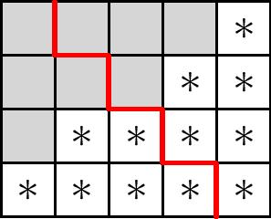
We first introduce some notation and terminology. Given two partitions $\lambda$ and $\nu$ with the Young diagram of $\lambda$ contained in that of $\nu$, we define $\nu/\lambda$ to be the skew shape formed by removing $\lambda$’s boxes from $\nu$. A semistandard Young tableau (SSYT) of shape $\nu/\lambda$ is a way of filling these boxes with positive integers so that the numbers are weakly increasing across rows and strictly increasing down columns. We say the SSYT has content $\mu$ if there are $\mu_i$ boxes labeled $i$ in the tableau for each $i$. The reading word of the tableau is the word formed by reading the entries in each row from left to right, starting with the bottom row and working towards the top. A word is lattice if every suffix has at least as many $i$’s as $i+1$’s for all $i$.
The following example shows a semistandard Young tableau of shape $\nu/\lambda$ where $\lambda=(2,2)$ and $\nu=(4,3,1)$. Its reading word is $1211$, which is lattice. Its content is $\mu=(3,1)$.
(Littlewood-Richardson rule.) For any two partitions $\lambda$ and $\mu$ contained in the Important Box, \[\sigma_\lambda\cdot\sigma_\mu =\sum c^\nu_{\lambda\mu} \sigma_\nu,\] where the sum ranges over all $\nu$ in the Important Box, and $c^\nu_{\lambda\mu}$ is the number of semistandard Young tableaux of shape $\nu/\lambda$ having content $\mu$ and whose reading word is lattice.
In his book, Fulton gives a full proof of this rule, by first proving the following special case.
(Pieri rule.) We have \[\sigma_\lambda\cdot \sigma_{(k)}=\sum_{\nu}\sigma_\nu\] where the sum ranges over all $\nu$ contained in the Important Box and such that $\nu/\lambda$ is a horizontal strip.
The Pieri rule is not hard to prove using some basic linear algebra (see Fulton, section 9.4), but the Littlewood-Richardson rule is much harder. For this, we turn to the hammer of symmetric function theory.
The combinatorics behind the rule: symmetric function theory
The Littlewood-Richardson and Pieri rules come up in symmetric function theory as well, and the combinatorics is much easier to deal with in this setting.
The ring of symmetric functions in infinitely many variables $x_1,x_2,\ldots$ is the ring \[\Lambda(x_1,x_2,\ldots)=\mathbb{C}[x_1,x_2,\ldots]^{S_\infty}\] of formal power series having bounded degree which are symmetric under the action of the infinite symmetric group on the indices.
For instance, $x_1^2+x_2^2+x_3^2+\cdots$ is a symmetric function, because interchanging any two of the indices does not change the series.
The most important symmetric functions in this context are the Schur functions. They can be defined in many equivalent ways, from being characters of irreducible representations of $\mathrm{GL}_n$ to an expression as a ratio of determinants. We use the combinatorial definition here, since it is most relevant to this context.
Let $\lambda$ be a partition. Given a semistandard Young tableau $T$ of shape $\lambda$, define $x^T=x_1^{m_1}x_2^{m_2}\cdots$ where $m_i$ is the number of $i$’s in the tableau $T$.
The Schur functions are the symmetric functions defined by \[s_\lambda=\sum_{T} x^T\] where the sum ranges over all SSYT’s $T$ of shape $\lambda$.
It is known that the Schur functions are symmetric, they form a basis of $\lambda_\mathbb{C}$, and they satisfy the Littlewood-Richardson rule: (see Fulton) \[s_\lambda\cdot s_\mu=\sum_{\nu} c^{\nu}_{\lambda\mu} s_\nu\] the only difference being that here, the sum is not restricted by any Important Box. It follows that there is a surjective ring homomorphism \[\Lambda(x_1,x_2,\ldots)\to H^\ast(\mathrm{Gr}^n(\mathbb{C}^m)))\] sending $s_\lambda\mapsto \sigma_\lambda$ if $\lambda$ fits inside the Important Box, and $s_\lambda\mapsto 0$ otherwise.
In particular, this means that any relation involving symmetric functions translates to a relation on $H^\ast(\mathrm{Gr}^n(\mathbb{C}^m))$. This connection makes the combinatorial study of symmetric functions an essential tool in Schubert calculus.
Examples
Example 1. Let’s compute $\sigma_{(1,1)}\cdot \sigma_{(2)}$ in $H^\ast(\mathrm{Gr}^2(\mathbb{C}^4))$. The Littlewood-Richardson rule tells us that the only possible $\nu$ must be the $2\times 2$ square $(2,2)$, but there is no way to fill $\nu/\lambda$ with two $1$’s in a semistandard way. Therefore, \[\sigma_{(1,1)}\cdot \sigma_{(2)}=0.\]
Geometrically, this makes sense: $\Omega_{(1,1)}$ is the Schubert variety consisting of all $2$-dimensional subspaces of $\mathbb{C}^4$ contained in a given $3$-dimensional subspace. $\Omega_{(2)}$ is the Schubert variety of all $2$-dimensional subspaces containing a given line through $0$. For a generic choice of the given $3$-dimensional subspace and line through the origin, there is plane satisfying both conditions.
Example 2. Let’s try the same calculation, $\sigma_{(1,1)}\cdot \sigma_{(2)}$, in $H^\ast(\mathrm{Gr}^3(\mathbb{C}^5))$. Now the Important Box is $2\times 3$, and so the partition $\nu=(3,1)$ is a possibility. Indeed, the Littlewood-Richardson rule gives us one possible filling of $\nu/\lambda$ with two $1$’s, and so we have \[\sigma_{(1,1)}\cdot \sigma_{(2)}=\sigma_{(3,1)}.\]
Geometrically, this also makes sense: $\Omega_{(1,1)}$ is the Schubert variety consisting of all $2$-dimensional subspaces of $\mathbb{C}^5$ contained in a given $4$-dimensional subspace. $\Omega_{(2)}$ is the Schubert variety of all $2$-dimensional subspaces intersecting a given plane through $0$ in at least a line. $\Omega_{(3,1)}$, then, is the variety of all $2$-dimensional subspaces contained in a given $4$-space and also containing a given line. Clearly the first and second conditions together are equivalent to the third in $\mathbb{C}^5$.
Example 3. We can now check in the least elegant possible way that there exists a unique line in projective space passing through two given points. In other words, through two given lines through $0$ in $\mathrm{Gr}^2(\mathbb{C}^3)$, we wish to show there is exactly one plane in the intersection of the varieties $\Omega_{(1)}$ and $\Omega_{(1)}$ (for two different flags). Our Important Box is $2\times 1$, so we have \[\sigma_{(1)}\cdot \sigma_{(1)}=\sigma_{(1,1)}.\] Indeed, $\Omega_{(1,1)}$ consists of a single plane in $\mathbb{C}^3$.
Example 4. We can now also solve problem 3. We wish to compute the product $\sigma_{(1)}^4$ in $H^\ast(\mathrm{Gr}^2(\mathbb{C}^4))$. We have $\sigma_{(1)}^2=\sigma_{(1,1)}+\sigma_{(2)}$ by the Littlewood-Richardson rule. Since $\sigma_{(1,1)}\cdot \sigma_{(2)}=0$ as in Example 1, we have \[\sigma_{(1)}^4=(\sigma_{(1,1)}+ \sigma_{(2)})^2=\sigma_{(1,1)}^2+\sigma_{(2)}^2=2\sigma_{(2,2)}.\] Thus there are exactly $2$ lines intersecting four given lines in $\mathbb{P}^3$.
Example 5. Finally, let’s solve problem 4 from the first page. The statement translates to proving a relation of the form \[\sigma_{(1)}^{r(m-r)}=c\cdot \sigma_{(n,n,\cdots, n)}\] where $c$ is the desired number of $r$-planes and the Schubert class on the right hand side refers to the class of the Important Box.
First note that some relation of this form must hold, since any partition $\nu$ on the right hand side of the product must have size $r(m-r)$ and fit in the Important Box. The Box itself is the only such partition.
To compute $c$, we notice that it is the same as the coefficient of $s_{(n,n,\ldots,n)}$ in the product of Schur functions $s_{(1)}^{rn}$ in the ring $\Lambda(x_1,x_2,\ldots)$. We now introduce some more well-known facts and definitions from symmetric function theory. (See Stanley’s or Sagan’s book to learn about symmetric functions in detail.)
Define the monomial symmetric function $m_\lambda$ to be the sum of all monomials in $x_1,x_2,\ldots$ having exponents $\lambda_1,\ldots,\lambda_r$. Then it is not hard to see, from the combinatorial definition of Schur functions, that \[s_\lambda=\sum_{\mu} K_{\lambda\mu} m_\mu\] where $K_{\lambda\mu}$ is the number of semistandard Young tableaux of shape $\lambda$ and content $\mu$. The numbers $K_{\lambda\mu}$ are called the Kostka numbers, and they can be thought of as a change of basis matrix in the space of symmetric functions.
The homogeneous symmetric function $h_\lambda$ is defined to be $h_{\lambda_1}\cdots h_{\lambda_r}$ where $h_d$ is the sum of all monomials of degree $d$ for any given $d$. The homogeneous symmetric functions also form a $\mathbb{C}$-basis for $\Lambda(x_1,x_2,\ldots)$, and one can then define an inner product on $\Lambda$ such that \[\langle h_\lambda,m_\mu\rangle=\delta_{\lambda\mu},\] i.e. the $h$’s and $m$’s are orthonormal. Remarkably, the $s_\lambda$’s are orthogonal with respect to this inner product: \[\langle s_\lambda,s_\mu\rangle=\delta_{\lambda\mu},\] and so we have \begin{eqnarray*} \langle h_\mu,s_\lambda\rangle &=& \langle h_\mu, \sum_{\nu} K_{\lambda\nu} m_\nu\rangle\\ &=& \sum_{\nu} K_{\lambda\nu}\langle h_\mu, m_\nu \rangle \\ &=& \sum_{\nu} K_{\lambda\nu} \delta{\mu\nu} \\ &=& K_{\lambda\mu} \end{eqnarray*} Thus we have the dual formula \[h_\mu=\sum_{\lambda}K_{\lambda\mu}s_\mu.\]
Returning to the problem, notice that $s_{(1)}=m_{(1)}=h_{(1)}=x_1+x_2+x_3+\cdots$. Thus $s_{(1)}^{rn}=h_{1}^{rn}=h_{(1,1,1,\ldots,1)}$ where the last vector has length $rn$. It follows from the formula above that the coefficient of $s_{(n,n,\cdots,n)}$ in $h_{(1,1,1,\ldots,1)}$ is the number of fillings of the Important Box with content $(1,1,1,\ldots,1)$, i.e. the number of Standard Young tableaux of Important Box shape.
There is a well-known and hard-to-prove theorem known as the hook length formula which will finish the computation.
Define the hook length $\mathrm{hook}(s)$ of a square $s$ in a Young diagram to be the number of squares strictly to the right of it in its row plus the number of squares strictly below in its column plus $1$ for the square itself.
(Hook length formula.) The number of standard Young tableaux of shape $\lambda$ is \[\frac{|\lambda|!}{\prod_{s\in \lambda}\mathrm{hook}(s)}.\]
Applying the hook length formula to the Important Box yields the total of \[\frac{(r(m-r))!\cdot (r-1)!\cdot (r-2)!\cdot \cdots\cdot 1!}{(m-1)!\cdot(m-2)!\cdot\cdots\cdot 1!}\] standard fillings, as desired.