Moduli of Curves I: A Curious Curve Count

Young tableaux are to planes as labeled trees are to curves. This is the analogy from which I hope to start a series of posts on the beauty of the growing field of connections between the geometry of moduli spaces of curves, and combinatorics.

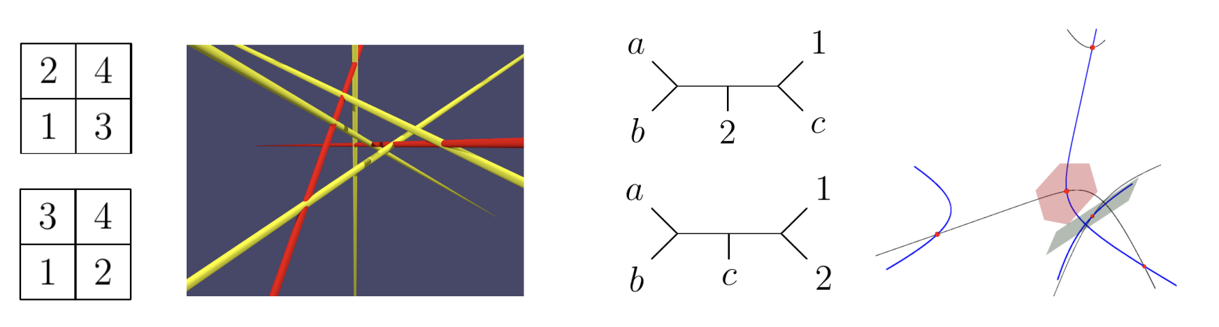
What do the pictures above have in common?

Two concrete questions

On the “planes” side of things, more commonly known as Schubert calculus (the study of linear intersection problems), one of the most famous and accessible examples that it can solve is the following:

QUESTION 1: Given four lines in 3 dimensional space, how many lines pass through all four of them?

In complex projective space, for a generic choice of four lines, the answer is 2, as shown by the red lines above. To deduce this using standard analytic/geometric methods alone is possible but cumbersome; the equations involved lead to a quadratic equation when solved, which has two solutions in general. But the magic of Schubert calculus is that that “2” can be computed as a much simpler combinatorial calculation:

QUESTION 1 (equivalent version in combinatorics): How many ways can the numbers 1, 2, 3, 4 be placed in the squares of a $2\times 2$ grid such that the numbers increase left to right in each row, and bottom to top in each column?

The two arrangements, called Young tableaux, are shown above at left. There are also other combinatorial solutions now as well, such as Knutson-Tao puzzles (shown above at right, also the two corresponding to the solution to Question 1) and Schubert calculus is the art of building a dictionary between combinatorial operations, invariants, and algorithms and the corresponding geometric properties in intersection theory.

On the “curves” side, here is a similarly concrete question one can formulate, that can be solved using algebraic and enumerative techniques in the theory of moduli spaces of curves:

QUESTION 2: Given 5 points $p_1, p_2, p_3, p_4, p_5$ in 3 dimensional space, a plane $P_1$ passing through $p_1$, and a plane $P_2$ passing through $p_2$, how many degree 3 curves pass through all 5 points and are tangent to planes $P_1$ and $P_2$ at $p_1$ and $p_2$ respectively?

The answer is also, coincidentally, 2! (For generic choices of points and planes, over complex projective space.) An example of 5 points in red, two planes, and the two curves (in black and blue) is shown below, with the full curves shown on the right, and zoomed in on the points shown at left:

Just as in Schubert calculus, there is an abstract way of figuring out the generic answer of “2” via intersection theory and associated combinatorics. Instead of Young tableaux and puzzles, we have parking functions and trees. At left below are the two standard parking functions of shape $(1,1)$, and at right are the two trivalent “slide trees” shown to correspond to this intersection problem in this paper.

Can intersection theory for curves be put on a rigorous combinatorial foundation as successfully as Schubert calculus has? Mumford stated this hope way back in his 1983 paper “Towards an Enumerative Geometry of the Moduli Space of Curves”:

The goal of this paper is to formulate and to begin an exploration of the enumerative geometry of the set of all curves of arbitrary genus $g$. […] We take as a model for this the enumerative geometry of the Grassmannians.

Much progress has been made since Mumford’s initial vision, and we aim to lay out what has been done so far, and what still needs to be done, in this sequence of posts.

The moduli spaces $M_{0,n}$ and $\overline{M}_{0,n}$

In order to get a handle on problems like Question 2, we first consider the question without the two tangent planes: how many degree 3 curves pass through the 5 given points in 3-space? The answer is now infinitely many, and in fact we have a two-parameter family of such curves. This defines a two-dimensional moduli space, which Kapranov showed is isomorphic to the space $M_{0,n}$. The latter, we explored briefly in this previous post. If we allow our cubics to be degenerate, such as a line through two of the points union with a plane through three, then the solutions are parameterized by the Deligne-Mumford compactification $\overline{M}_{0,n}$.

We recall the definition here: $M_{0,n}$, for $n\ge 3$, is the set of all ways of choosing $n$ distinct points $p_1,\ldots,p_n$ on the projective line $\mathbb{P}^1$, up to isomorphism. Note that a linear projective transformation of $\mathbb{P}^1$ is determined by where it sends three points, and so by only considering the configurations up to isomorphism, we may equivalently fix three of the points $p_1,p_2,p_3$ to be $(0:1),(1:1),(1:0)$ (in other words, $0,1,\infty$) and then the remaining $n-3$ points may be any other distinct points on the curve.

In fact, this means $M_{0,3}$ contains exactly one element. Historically, the notion of moduli spaces of curves stemmed from the attempt to classify complex Riemann surfaces according to their genus $g$, which is the number of holes:

(Picture taken from Sean Carroll’s lecture notes on General Relativity.)

The fact that $M_{0,3}$ is a single point is simply saying that any connected, smooth genus $0$ Riemann surface is isomorphic to $\mathbb{P}^1$, and marking three of the points removes its own automorphism group for simplicity. But now what if we add more marked points? There is a way that we can turn the set $M_{0,n}$ into a topological space, where for instance the space $M_{0,5}$ is two dimensional, because the two points $p_4,p_5$ are each chosen from a one-dimensional space. Formally, we can view $M_{0,5}$ as a subset of $\mathbb{P}^1\times \mathbb{P}^1$ and inherit the subspace topology. In general, then:

$\overline{M}_{0,n}$ has dimension $n-3$.

Note that we haven’t specified what field we are working over in any of this; we will usually be implicitly working over $\mathbb{C}$, even though our pictures may be over $\mathbb{R}$, as in the example of the cubic above.

The first thing one will notice when trying to study $\overline{M}_{0,n}$ as a space is that there are “holes” in it. For instance, for $\overline{M}_{0,4}$, we may think of three points as fixed on $\mathbb{P}^1$ and a fourth point moving freely around the circle (or sphere, if we are over $\mathbb{C}$. However, what happens when the fourth point approaches one of the three fixed points? There are various compactifications that fill these holes, and we will discuss many of them in future posts. For now, for $\overline{M}_{0,4}$, the three holes may be closed up by allowing the fourth point $p_4$ to collide with another point, say $p_1$, by creating a new $\mathbb{P}^1$ attached at a node the location of $p_1$ that contains $p_1,p_4$, with the other $\mathbb{P}^1$ still containing $p_2,p_3$.

Psi classes

For the Schubert calculus problem with four lines, we saw in previous posts that we can rephrase it in terms of the intersection product of Schubert classes \[\int_{\mathrm{Gr}(2,4)} \sigma_1^4=2.\] For the curves problem, we can phrase it as an intersection product of psi classes on $\overline{M}_{0,n}$. Indeed, a psi class $\psi_i$ in the Chow ring of $\overline{M}_{0,n}$ encodes the differential information to the curves at the point $i$, and under Kapranov’s correspondence, it enforces a tangent plane condition at point $i$. Thus the computation can be translated as \[\int_{\overline{M}_{0,5}} \psi_1\psi_2=2.\]

In general, it is known that \[\int_{\overline{M}_{0,n+3}} \psi_1^{k_1}\cdots \psi_n^{k_n}=\binom{n}{k_1,\ldots,k_n}=\frac{n!}{k_1!\cdots k_n!},\] where the $k_i$’s sum to $n$. Thus if we instead put two tangent plane conditions at a single one of the 5 points instead of two different points, requiring a specific tangent line at the first point, we are computing $\int_{\overline{M}_{0,5}} \psi_1^2=1$. Thus there is exactly one cubic through $5$ given points and tangent to a given line at one of the points, in general.

A simpler example and $\overline{M}_{0,4}$

Consider the following simpler setup than Question 2:

QUESTION 3: Given 4 points $p_1, p_2, p_3, p_4$ in the plane and a line through $p_1$, how many conics pass through all four points and are tangent to the given line?

The answer here is $1$, and we can see this quite easily in a concrete example. Choose the four points to be $(1,1)$, $(1,-1)$, $(-1,-1)$, $(-1,1)$. Then certainly the circle $x^2+y^2=2$ passes through all four of them, as does any quadratic of the form \[ax^2+(2-a)y^2=2\] for any nonzero constant $a$. In real space, we then have that:

When $0\lt a\lt 2$, we have an ellipse through the points, with $a=1$ giving the circle.
When $a=0$ we have the degenerate situation of two horizontal parallel lines, $x=\pm 1$.
When $a=2$ it is two vertical lines, $y=\pm 1$.
When $a\gt 2$, we have a hyperbola with a left and right branch.
When $a\lt 0$ we have a hyperbola with a top and bottom branch.
In between the two previous cases, at the degenerate point $a=\infty$ (or $-\infty$), we have the two crossing lines $x=y$ and $x=-y$.

This is all shown in the animation below.

Note that the tangent line at $(1,1)$ to the quadratic has slope $a/(a-2)$ (it is a fun exercise to do this with calculus, and even more fun to do it without solving for $y$ first). This changes with the value of $a$, and in particular there is only one conic through the four points for each slope $a$. To prove this rigorously, one may consider an arbitrary conic \[ax^2+bxy+cy^2+dx+ey+f=0\] and, given that it passes through $(\pm 1,\pm 1)$, show algebraically by solving the linear equations that $a+c=f=2$ and the other coefficients must be $0$. We leave this as an exercise for the reader.

What does this all demonstrate? That a single $\psi$ class on $\overline{M}_{0,4}$ has intersection number $1$. Beautiful!

Appendix on the construction of the two curves

The pictures above, showing the two cubics through 5 given points and tangent to two given planes, is difficult to construct mathematically and plot; sometimes the solutions will be complex, or sometimes we will accidentally land in a degenerate case. To find a plottable situation with two real solutions, we constructed the curves mathematically as follows.

Let’s first consider the problem in complex projective $3$-space, so we are working in $\mathbb{P}^3$, with homogeneous coordinates $(x:y:z:w)$. Let us consider the $5$ points:

$(1:0:0:0)$
$(0:1:0:0)$
$(0:0:1:0)$
$(0:0:0:1)$
$(1:1:1:1)$

The first three of these points are “at infinity” with $w=0$, but we can later apply a projective transformation so that the 5 points are all at finite coordinates in the affine patch $(x:y:z:1)$ and therefore plottable in 3D.

It is not hard to construct a generic parameterized cubic passing through these five points, with respect to a parameter $t$, that passes through the $5$ points at values $t_1,t_2,t_3,t_4,t_5$ respectively. The general form is:

\[\vec{f}(t)=\left(\frac{t_5-t_1}{t-t_1}:\frac{t_5-t_2}{t-t_2}:\frac{t_5-t_3}{t-t_3}:\frac{t_5-t_4}{t-t_4}\right).\]

A quick inspection shows that this passes through the $5$ points as claimed, and it is cubic because if we multiply through by the denominators, each coordinate is a cubic polynomial in $t$.

Now, the parameter $t$ is from $\mathbb{P}^1$, which is only determined up to automorphism by where it sends $3$ points. (Note that technically we might have written $\vec{f}(t:1)=\cdots$, and understood that as $t\to \infty$ we get $\vec{f}(1:0)$.) We can therefore make choices for $t_3,t_4,t_5$, where we will avoid choosing infinity or complex numbers in order to again make things plottable. Let us conveniently choose $t_5=0$, $t_4=1$, $t_3=2$. Then we have

\[\vec{f}(t)=\left(\frac{1-t_1}{t-t_1}:\frac{1-t_2}{t-t_2}:\frac{-1}{t-2}:\frac{1}{t}\right)\]

We can multiply through by $t$ to clear the last denominator and get into an affine chart. We also rename $t_1,t_2$ to $a,b$ respectively for readability:

\[\vec{f}(t)=\left(\frac{t(1-a)}{t-a}:\frac{t(1-b)}{t-b}:\frac{t}{2-t}:1\right)\]

Now, we wish to choose two planes with real normal vectors and impose the tangent conditions, so that there are exactly two distinct pairs of real solutions for $a$ and $b$. We can write down

$rx+sy+z=0$ and
$mx+ny+z=0$ as our two tangent planes at the real points $(0,0,0)$ and $(1,1,1)$ respectively, where $r,s,m,n$ will be constants, and note that in the affine patch $(x:y:z:1)$, we can reduce to three affine coordinates and compute the tangent direction at $t$:

\[\vec{f}’(t)= \left(\frac{a^2-a}{(t-a)^2}, \frac{b^2-b}{(t-b)^2},\frac{2}{(2-t)^2}\right)\]

Thus at $t=0$, at which $f(t)=(0,0,0)$, we have

\[\vec{f}’(0)= \left(\frac{a-1}{a}, \frac{b-1}{b},\frac{1}{2}\right)\]

and at $t=1$, at which $f(t)=(1,1,1)$, we have

\[\vec{f}’(1)= \left(\frac{a}{1-a}, \frac{b}{1-b},2\right)\]

At $t=0$ we wish this vector to lie in the first plane, and at $t=1$ we wish it to lie in the second. Plugging these into Sage and solving for $a,b$ we find:

In other words, we do generically get two solutions, since the equation becomes quadratic in $a,b$, and the discriminant is

\[m^2r^2+n^2s^2-2mr-2mnrs-2ns+1.\]

In order to have distinct real solutions, we need to choose $r,s,m,n$ such that this discriminant is a positive real number. Let’s in fact try to make the discriminant be $1$; this will cancel the constant term, and in fact we will find rational solutions $a,b$. I played around with some values until I found that setting $s=1,r=-1$ makes for a nice discriminant, and we now want:

\[m^2+n^2+2m+2mn-2n=0\]

which can be rewritten as

\[(n+m)^2=2(n-m)\]

and so we can pick $n,m$ such that $n+m=1$ and $n-m=1/2$, in other words, $m=1/4$ and $n=3/4$. Asking Sage again, this makes $a,b$ have the following two solutions:

$(a,b)=(4/3,4/5)$
$(a,b)=(4/5,4/7)$

Plugging this all back in, what have we found?

For tangent planes

$-x+y+z=0$ at $(0,0,0)$
$x+3y+4z=8$ at $(1,1,1)$

there are exactly two cubic curves passing through $(0,0,0)$ and $(1,1,1)$ and approaching the other three points at infinity in projective space, and tangent to these two planes. They are

$\vec{f}(t)=\left(\frac{t}{4-3t},\frac{t}{5t-4},\frac{t}{2-t}\right)$
$\vec{g}(t)=\left(\frac{t}{5t-4},\frac{3t}{7t-4},\frac{t}{2-t}\right)$

Indeed, re-projectivizing by adding the $w=1$ coordinate at the end, we have

$\vec{f}(4/3)=\vec{g}(4/5)=(1:0:0:0)$
$\vec{f}(4/5)=\vec{g}(4/7)=(0:1:0:0)$
$\vec{f}(2)=\vec{g}(2)=(0:0:1:0)$
$\vec{f}(0)=\vec{g}(0)=(0:0:0:1)$
$\vec{f}(1)=\vec{g}(1)=(1:1:1:1)$

And the tangent conditions are satisfied as above. We now perform a projective linear transformation $(x:y:z:w)\mapsto (x:y:z:x+y+z+w)$ so that the new set of five points is

$(1:0:0:1)$
$(0:1:0:1)$
$(0:0:1:1)$
$(0:0:0:1)$
$(1/4:1/4:1/4:1)$

where we have renormalized the last point so all have $w=1$ again. We similarly apply this transformation to the formulas for $\vec{f}$ and $\vec{g}$, and divide through by the $w$ term, and then get the following transformed formulas for $f$ and $g$:

$\vec{f}(t)=(t(5t-4)(2-t)/d,t(4-3t)(2-t)/d, t(4-3t)(5t-4)/d)$ where $d=-2t^3 -26t^3 + 64t -32$,
$\vec{g}(t)=(t(7t-4)(2-t)/D,3t(5t-4)(2-t)/D, t(5t-4)(7t-4)/D)$ where $D=-22t^3 + 130t^3- 128t + 32$,

and we can plot these in Asymptote or using any other 3D plotting tool to get this done. One question I still have is:

How can we algorithmically construct real intersection solutions to $\psi$ class products in general?

Thanks to Jake Levinson for helping with this explicit curve construction.