
The Springer Correspondence Part IV: Affine Springer Fibers
I have written about the flag variety, the Springer resolution, and the relation between the type A Springer correspondence and Hall-Littlewood polynomials in a previous sequence of posts.
Time to extend this construction to the (type A) affine flag variety, corresponding to affine Lie type $\widetilde{A}_n$! We’ll also see how, due to a result of Hikita in 2012, this construction gives rise to a geometric interpretation of the famous symmetric functions $\nabla e_n$ from the Shuffle theorem.
What is an affine flag?
Recall that a classical flag is a chain of subspaces:
\[0=V_0\subset V_1 \subset V_2 \subset \cdots \subset V_n=\mathbb{C}^n\]
with $\dim V_i=i$ for all $i$.
An affine flag is a chain of lattices over the ring $\mathbb{C}[[\epsilon]]$ in the space $\mathbb{C}((\epsilon))^n$. We write $\mathbb{F}=\mathbb{C}((\epsilon))$ for the field of Laurent series in the variable $\epsilon$ over $\mathbb{C}$, whose elements generally look something like:
\[\epsilon^{-3}+\epsilon^{-1}+1-\epsilon - 3\epsilon^2+ \epsilon^3 +\cdots \in \mathbb{F}\]We also write $\mathbb{O}=\mathbb{C}[[\epsilon]]$ for the ring of formal power series in $\epsilon$, whose elements generally look something like:
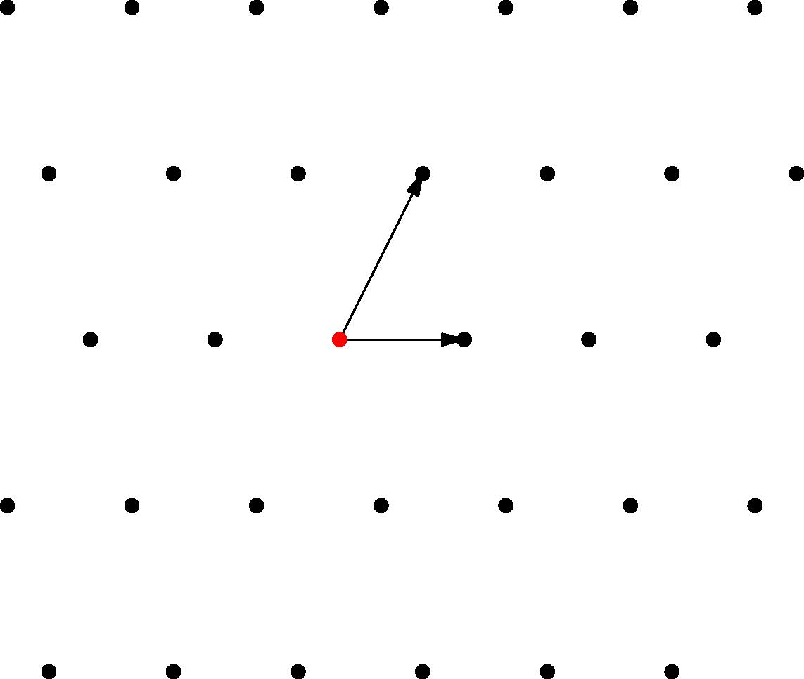
\[1+2\epsilon+3\epsilon^2-7\epsilon^3+\cdots\in \mathbb{O}.\]An $\mathbb{O}$-lattice $\Lambda\subseteq \mathbb{F}^n$ is the $\mathbb{O}$-span of a set of $n$ independent vectors in $\mathbb{F}^n$. It is called a lattice because of the similar setting of $\mathbb{Z}$-lattices in $\mathbb{R}^2$, which consists of the integer linear combinations of two independent vectors in the plane:
Finally, an affine flag is a chain
\[\Lambda_1\subseteq \Lambda_2\subseteq \cdots \subseteq \Lambda_n\subseteq \mathbb{F}^n\]of nested lattices such that
\[\epsilon\Lambda_n\subseteq \Lambda_1.\]Standard affine flag and $\mathrm{GL}_n(\mathbb{F})$ action
Here is an example: suppose $v_1,\ldots, v_n$ is the standard basis of $\mathbb{F}^n$, where $v_i$ is the column vector with a $1$ in the $i$th position and $0$ elsewhere. Then the standard flag $\Lambda^{\mathrm{std}}_\bullet$ is defined by
\[\begin{align*} \Lambda_1^{\mathrm{std}} &= \mathbb{O}\{v_1, \epsilon v_2, \epsilon v_3,\epsilon v_4, \ldots, \epsilon v_n\} \\ \Lambda_2^{\mathrm{std}} &= \mathbb{O}\{v_1,v_2, \epsilon v_3, \epsilon v_4, \ldots, \epsilon v_n\} \\ \Lambda_3^{\mathrm{std}} &= \mathbb{O}\{v_1,v_2, v_3, \epsilon v_4, \ldots, \epsilon v_n\} \\ \vdots & \\ \Lambda_n^{\mathrm{std}} &= \mathbb{O}\{v_1,v_2, v_3, v_4, \ldots, v_n\} \\ \end{align*}\]and note that \(\epsilon \Lambda_n^{\mathrm{std}}=\mathbb{O}\{\epsilon v_1,\epsilon v_2,\epsilon v_3,\epsilon v_4, \ldots, \epsilon v_n\} \subseteq \Lambda_1^{\mathrm{std}},\) so this is a well-defined affine flag.
We now consider the action of $\mathrm{GL}_n(\mathbb{F})$ on the chains of lattices; notice that multiplying each $\Lambda_i$ space by an invertible matrix $g$ results in another affine flag, and that the action is transitive. We now compute the stabilizer of $\Lambda_\bullet^{\mathrm{std}}$. We claim that it is actually a subgroup of $\mathrm{GL}_n(\mathbb{O})$, and consists of precisely the matrices $M(\epsilon)$ such that setting $\epsilon=0$ yields an upper-triangular invertible matrix $M(0)$. That is, they have the form (for $n=4$ below):
\[\begin{pmatrix} \star & \ast & \ast & \ast \\ \epsilon \ast & \star & \ast & \ast \\ \epsilon \ast & \epsilon \ast & \star & \ast \\ \epsilon \ast & \epsilon \ast & \epsilon \ast & \star \end{pmatrix}\]where the $\star$’s must have a nonzero constant term and the $\ast$’s can be any element of $\mathbb{O}$.
Indeed, note that any such matrix stabilizes each lattice $\Lambda^{\mathrm{std}}_i$, since it replaces each $v_i$ with a linear combination of $v_j$’s for $j\le i$ and $\epsilon v_k$’s for $k\ge i$. Conversely, we cannot have any $\epsilon^{-1}$ terms (or lower) appearing in the matrix, for then some basis element would have an $\epsilon^{-1}v_i$, which does not appear in any $\Lambda^{\mathrm{std}}$ piece. And the lower elements must be divisible by $\epsilon$ in order to preserve each $\Lambda_i^{\mathrm{std}}$, with the entire matrix still being invertible; the result follows.
Finally, we write $I_n$ for the stabilizer, called the Iwahori subgroup. This is the analog of the Borel subgroup for the ordinary flag variety. Thus for instance,
\[I_4= \begin{pmatrix} \star & \ast & \ast & \ast \\ \epsilon \ast & \star & \ast & \ast \\ \epsilon \ast & \epsilon \ast & \star & \ast \\ \epsilon \ast & \epsilon \ast & \epsilon \ast & \star \end{pmatrix}.\]Algebraic definition of affine flag variety
Since $\mathrm{GL}_n(\mathbb{F})$ acts transitively on affine flags and the stabilizer of $\Lambda_\bullet^{\mathrm{std}}$ is $I_n$, we can naturally associate each affine flag to a coset $gI_n$. This leads to the algebraic definition of the affine flag variety:
\[\widetilde{\mathrm{Fl}}_n=\mathrm{GL}_n(\mathbb{F})/I_n.\]Thus, an affine flag can be thought of as an equivalence class of matrices up to the right action of $I_n$, and we can take a canonical representative by performing modified row reduction operations as follows. One set of generators for the Iwahori subgroup $I_n$ consists of matrices of the following three types:
\[\begin{pmatrix} 1 & 0 & 1 & 0 \\ 0 & 1 & 0 & 0 \\ 0 & 0 & 1 & 0 \\ 0 & 0 & 0 & 1 \end{pmatrix} \hspace{2cm} \begin{pmatrix} 1 & 0 & 0 & 0 \\ 0 & 1 & 0 & 0 \\ 0 & \epsilon & 1 & 0 \\ 0 & 0 & 0 & 1 \end{pmatrix} \hspace{2cm} \begin{pmatrix} a & 0 & 0 & 0 \\ 0 & b & 0 & 0 \\ 0 & 0 & c & 0 \\ 0 & 0 & 0 & d \end{pmatrix}\]where at left, the $1$ can be anywhere in the upper right, at middle the $\epsilon$ can be anywhere in the lower left, and $a,b,c,d$ are any invertible elements of $\mathbb{O}$.
This means that the three elementary matrix operations that preserve the affine flag represented by a matrix are:
- Scaling a column by an invertible element from $\mathbb{O}$, that is, a power series in $\epsilon$ that has a nonzero constant term,
- Adding a column to a column to its right,
- Adding $\epsilon$ times a column to a column to the left.
Note that by combining these operations, we can in fact add any $\mathbb{O}$-scalar multiple of column $i$ to column $j$ to its right, and any $\epsilon \mathbb{O}$-scalar multiple of a column to its left, even if those scalars are not invertible, since we can add two invertible scalars to get an arbitrary scalar.
Thus we can perform the following row reduction algorithm to any matrix and obtain a canonical affine flag representative:
- Consider the valuation of each element of the top row, meaning the minimum power of $\epsilon$ appearing in each Laurent series. Among all entries with smallest valuation $v$ in that row, choose the leftmost as the pivot in the top row.
- Use column operations to clear the elements to its left and right.
- Scale the pivot column by an invertible element so that its value is simply $\epsilon^{-v}$.
- Repeat steps 1-3 on the second row and beyond, where we only consider the entries that are not underneath a pivot above at each step.
For instance, suppose we start with the matrix
\[\begin{pmatrix} 1 & \epsilon^{-1} & 0 & \epsilon^{-1}-1 \\ \epsilon & 1 & \epsilon & 2-\epsilon \\ 1 & 0 & -2 & 0 \\ \epsilon^{-2}+\epsilon^3 & \epsilon^2 & -2\epsilon^{-2}+\epsilon^2+\epsilon^4 & \epsilon^2 \end{pmatrix}\](where we keep in mind that in general the entries may be infinite power series). The pivot in the top row is in the second column, with valuation $-1$, and we can subtract $\epsilon$ times column $2$ from column $1$, and subtract $1-\epsilon$ times column $2$ from column $4$. This yields:
\[\begin{pmatrix} 0 & \epsilon^{-1} & 0 & 0 \\ 0 & 1 & \epsilon & 1 \\ 1 & 0 & -2 & 0 \\ \epsilon^{-2} & \epsilon^2 & -2\epsilon^{-2}+\epsilon^2+\epsilon^4 & \epsilon^3 \end{pmatrix}\]Then, the pivot in the second row is the rightmost $1$, and we clear the third column to its left:
\[\begin{pmatrix} 0 & \epsilon^{-1} & 0 & 0 \\ 0 & 1 & 0 & 1 \\ 1 & 0 & -2 & 0 \\ \epsilon^{-2} & \epsilon^2 & -2\epsilon^{-2}+\epsilon^2 & \epsilon^3 \end{pmatrix}\]The pivot in the third row is then the leftmost entry, which we use to clear the $-2$, and obtain:
\[\begin{pmatrix} 0 & \epsilon^{-1} & 0 & 0 \\ 0 & 1 & 0 & 1 \\ 1 & 0 & 0 & 0 \\ \epsilon^{-2} & \epsilon^2 & \epsilon^2 & \epsilon^3 \end{pmatrix}\]The final pivot is then the $\epsilon^2$ in the third column, which can be used to clear the entry to its right:
\[\begin{pmatrix} 0 & \epsilon^{-1} & 0 & 0 \\ 0 & 1 & 0 & 1 \\ 1 & 0 & 0 & 0 \\ \epsilon^{-2} & \epsilon^2 & \epsilon^2 & 0 \end{pmatrix}\]If the matrix above is $g$, this represents the affine flag $g\Lambda^{\mathrm{std}}_\bullet$. For instance, the first piece of this flag is
\[g\Lambda^{\mathrm{std}}_1=\mathbb{O}\{v_3+\epsilon^{-2}v_4, \epsilon^{-1}v_1+v_2+\epsilon^2 v_4,\epsilon^2 v_4, v_2\}.\]Schubert decomposition and affine permutations
In the above simplification, consider the matrix consisting of only the pivots:
\[\begin{pmatrix} 0 & \epsilon^{-1} & 0 & 0 \\ 0 & 0 & 0 & 1 \\ 1 & 0 & 0 & 0 \\ 0 & 0 & \epsilon^2 & 0 \end{pmatrix}\]This is an affine permutation matrix, which in general consists of a permutation matrix whose $1$’s are replaced by powers of $\epsilon$. This data corresponds to an affine permutation in the affine symmetric group $\widetilde{S}_n$. An affine permutation is defined as a bijective map $w:\mathbb{Z}\to \mathbb{Z}$ such that the numbers $w_1,\ldots,w_n$ each are in a different equivalence class modulo $n$ and
\[w_{i+n}=w_i + n\]for all $i$.
The window of an affine permutation is the sequence $[w_1,\ldots,w_n]$, which completely determines the rest of the bijection by adding $n$ each time we move $n$ steps to the right (or subtracting if we move $n$ steps left). Let $\pi_i$ be the residue of $w_i$ mod $n$ for all $i$; then $\pi$ is a permutation in the ordinary symmetric group $S_n$, and we can uniquely write $w_i=\pi_i+n\lambda_i$ for some integers $\lambda_i$ for each $i$. Then we define the action of an affine permutation on $\mathbb{F}^n$ by
\[w\cdot v_i=\epsilon^{\lambda_i}v_{\pi_i}\]and extending by linearity.
This action corresponds to that of the matrix whose $(\pi_i,i)$ entry is $\epsilon^{\lambda_i}$. Thus the affine permutation corresponding to the affine permutation matrix above is, in window notation,
\[[3,-3,12,2]\]which corresponds to the full affine permutation
\[\ldots,-1,-7,8,-2,[3,-3,12,2],7,1,16,6,\ldots\]and whose associated permutation $\pi$ is $3,1,4,2$.
Finally, the Schubert cell $C_w$ in the affine flag variety $\widetilde{\mathrm{Fl}}_n$ is the set of affine flags whose matrix of pivots corresponds to the affine permutation $w\in \widetilde{S}_n$. Clearly the disjoint union of Schubert cells is the entire variety. An inspection of the row reduction procedure can show that each cell is affine of dimension $\mathrm{inv}(w)$, where inv denotes the number of pairs $(i,j)$ with $i<j$, $w(i)>w(j)$, and $j$ an index in the window ($1\le j\le n$).
Diagonal coinvariants
In the post on the ordinary flag variety, we saw that the cohomology ring $H^\ast(\mathrm{Fl}_n)$ is equal to the one-variable coinvariant ring $R_n=\mathbb{Q}[x_1,\ldots,x_n]/(e_1,\ldots,e_n)$ where $e_i$ is the $i$-th elementary symmetric polynomial in the $n$ variables. That is, it is the quotient by the ideal generated by positive degree invariants under the natural action of $S_n$.
In two sets of variables, we have a diagonal action of $S_n$ on $\mathbb{Q}[x_1,\ldots,x_n,y_1,\ldots,y_n]$ by acting on the two sets of variables in parallel: $\pi\cdot x_i=x_{\pi(i)}$ and $\pi\cdot y_i=y_{\pi(i)}$. We can then similarly construct the diagonal coinvariant ring
\[\mathrm{DR}_n=\mathbb{Q}[x_1,\ldots,x_n,y_1,\ldots,y_n]/I\]where $I$ is the ideal generated by all positive-degree homogeneous invariants under the diagonal action.
The famous Shuffle conjecture – now the Shuffle Theorem due to Carlsson and Mellit – gave a combinatorial formula for the doubly graded Frobenius series of $\mathrm{DR}_n$, that is, a full decomposition into irreducible $S_n$ representations, broken down according to both $x$ and $y$ degree. There is also an important geometric interpretation of $\mathrm{DR}_n$ due to Haiman in the context of the Hilbert scheme of $n$ points in the plane.
We now will describe a different geometric interpretation of $\mathrm{DR}_n$ in terms of affine Springer fibers, due to Hikita.
Affine Springer fibers
An affine Springer fiber is defined in much the same way as a classical Springer fiber: we start with a matrix $\gamma$ (nilpotent in the classical case) and consider all flags fixed by $\gamma$. In this case, we specifically define
\[\gamma = \begin{pmatrix} 0 & \epsilon & 0 & 0 \\ 0 & 0 & \epsilon & 0 \\ 0 & 0 & 0 & \epsilon \\ \epsilon^2 & 0 & 0 & 0 \end{pmatrix}\]that in general has $\epsilon$’s on the off diagonal and $\epsilon^2$ in the lower left corner. Then define the affine springer fiber
\[B_\gamma = \{\Lambda_\bullet : \forall i, \gamma\Lambda_i \subseteq \Lambda_i \}.\]Hikita found an affine paving that leads to a second grading on the Borel-Moore homology $H_\ast^{BM}(B_\gamma)$, giving rise to a doubly-graded $S_n$-module that he calls $R_\gamma=\mathrm{gr}_\ast H_\ast^{BM}(B_\gamma)$. Then Hikita’s main theorem is that if we reverse the degrees of one of the two gradings on $R_\gamma$ and tensor by the sign representation, we obtain the same graded $S_n$ module as $\mathrm{DR}_n$! In Frobenius series language,
\[\mathrm{Frob}_{q,t}(R_\gamma)= \mathrm{rev}_q \circ \omega (\nabla e_n)\]where here $\nabla e_n$ is another name for the Frobenius series of the diagonal coinvariant ring. Beautiful!