The Springer Correspondence, Part I: The Flag Variety
In prior posts, we’ve seen that the irreducible representations of the symmetric group $S_n$ are in one-to-one correspondence with the partitions of $n$, and the Schur functions give an elegant encoding of their characters as symmetric polynomials. Now we can dive a bit deeper: a geometric construction known as the Springer resolution allows us to obtain all the irreducible representations of $S_n$ geometrically, and as a side bonus give natural graded representations that will allow us to define a $q$-analog of the Schur functions known as the Hall-Littlewood polynomials.
Quite a mouthful of terminology. Let’s start at the beginning.
The Classical Flag Variety
When you think of a flag, you might imagine something like this:
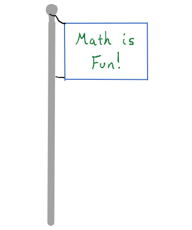
Roughly speaking, a flag on a flagpole consists of:
- a point (the bulbous part at the top of the pole),
- a line passing through that point (the pole),
- a plane passing through that line (the plane containing the flag), and
- space to put it in.
Mathematically, this is the data of a complete flag in three dimensions. However, higher-dimensional beings would require more complicated flags. So in general, a complete flag in $n$-dimensional space $\mathbb{C}^n$ is a chain of vector spaces of each dimension from $0$ to $n$, each containing the previous:
\[0=V_0\subset V_1 \subset V_2 \subset \cdots \subset V_n=\mathbb{C}^n\]
with $\dim V_i=i$ for all $i$.
(Our higher-dimensional flag-waving imaginary friends are living in a world of complex numbers because $\mathbb{C}$ is algebraically closed and therefore easier to work with. However, one could define the flag variety similarly over any field $k$.)
Variety Structure
Now that we’ve defined our flags, let’s see what happens when we wave them around continuously in space. It turns out we get a smooth algebraic variety!
Indeed, the set of all possible flags in $\mathbb{C}^n$ forms an algebraic variety of dimension $n(n-1)$ (over $\mathbb{R}$), covered by open sets similar to the Schubert cells of the Grassmannian. In particular, given a flag $\{V_i\}_{i=1}^n$, we can choose $n$ vectors $v_1,\ldots,v_n$ such that the span of $v_1,\ldots,v_i$ is $V_i$ for each $i$, and list the vectors $v_i$ as row vectors of an $n\times n$ matrix. We can then perform certain row reduction operations to form a different basis $v_1^\prime,\ldots,v_n^\prime$ that also span the subspaces of the flag, but whose matrix is in the following canonical form: it has $1$’s in a permutation matrix shape, $0$’s to the left and below each $1$, and arbitrary complex numbers in all other entries.
For instance, say we start with the flag in three dimensions generated by the vectors $\langle 0,2,3\rangle$, $\langle 1, 1, 4\rangle$, and $\langle 1, 2, -3\rangle$. The corresponding matrix is \[\left(\begin{array}{ccc} 0 & 2 & 3 \\ 1 & 1 & 4 \\ 1 & 2 & -3\end{array}\right).\] We start by finding the leftmost nonzero element in the first row and scale that row so that this element is $\newcommand{\PP}{\mathbb{P}} \newcommand{\CC}{\mathbb{C}} \newcommand{\RR}{\mathbb{R}} \newcommand{\ZZ}{\mathbb{Z}} \DeclareMathOperator{\Gr}{Gr} \DeclareMathOperator{\Fl}{F\ell} \DeclareMathOperator{\GL}{GL} \DeclareMathOperator{\inv}{inv}1$. Then subtract multiples of this row from the rows below it so that all the entries below that $1$ are $0$. Continue the process on all further rows:
\[\left(\begin{array}{ccc} 0 & 2 & 3 \\ 1 & 1 & 4 \\ 1 & 2 & -3\end{array}\right) \to \left(\begin{array}{ccc} 0 & 1 & 1.5 \\ 1 & 0 & 2.5 \\ 1 & 0 & -6\end{array}\right)\to \left(\begin{array}{ccc} 0 & 1 & 1.5 \\ 1 & 0 & 2.5 \\ 0 & 0 & 1\end{array}\right)\]
It is easy to see that this process does not change the flag formed by the partial row spans, and that any two matrices in canonical form define different flags. So, the flag variety is covered by $n!$ open sets given by choosing a permutation and forming the corresponding canonical form. For instance, one such open set in the $5$-dimensional flag variety is the open set given by all matrices of the form \[\left(\begin{array}{ccccc} 0 & 1 & \ast & \ast & \ast \\ 1 & 0 & \ast & \ast & \ast \\ 0 & 0 & 0 & 0 & 1 \\ 0 & 0 & 1 & \ast & 0 \\ 0 & 0 & 0 & 1 & 0 \end{array}\right)\] We call this open set $X_{45132}$ because it corresponds to the permutation matrix formed by placing a $1$ in the $4$th column from the right in the first row, in the $5$th from the right in the second row, and so on. The maximum number of $\ast$’s we can have in such a matrix is when the permutation is $w_0=n(n-1)\cdots 3 2 1$, in which case the dimension of the open set $X_{12\cdots n}$ is $n(n-1)/2$ over $\CC$ — or $n(n-1)$ over $\RR$, since $\CC$ is two-dimensional over $\RR$. In general, the number of $\ast$’s in the set $X_w$ is the inversion number $\inv(w)$, the number of pairs of entries of $w$ which are out of order.
Finally, in order to paste these disjoint open sets together to form a smooth manifold, we consider the closures of the sets $X_w$ as a disjoint union of other $X_w$’s. The partial ordering in which $\overline{X_w}=\sqcup_{v\le w} X_v$ is called the Bruhat order, a famous partial ordering on permutations. (For a nice introduction to Bruhat order, one place to start is Yufei Zhao’s expository paper on the subject.)
Cohomology
Now suppose we wish to answer incidence questions about our flags: which flags satisfy certain given constraints? As in the case of the Grassmannians, this boils down to understanding how the Schubert cells $X_w$ intersect. This question is equaivalent to studying the cohomology ring of the flag variety $\Fl_n$ over $\mathbb{Z}$, where we consider the Schubert cells as forming a cell complex structure on the flag variety.
The cohomology ring $H^\ast(\Fl_n)$, as it turns out, is the coinvariant ring that we discussed in the last post! For full details I will refer the interested reader to Fulton’s book on Young tableaux. To give the reader the general idea here, the Schubert cell $X_w$ can be thought of as a cohomology class in $H^{2i}(\Fl_n)$ where $i=\inv(w)$. We call this cohomology class $\sigma_w$, and note that for the transpositions $s_i$ formed by swapping $i$ and $i+1$, we have $\sigma_{s_i}\in H^2(\Fl_n)$. It turns out that setting $x_i=\sigma_i-\sigma_{i+1}$ for $i\le n-1$ and $x_n=-\sigma_{s_{n-1}}$ gives a set of generators for the cohomology ring, and in fact \[H^\ast(\Fl_n)=\mathbb{Z}[x_1,\ldots,x_n]/(e_1,\ldots,e_n)\] where $e_1,\ldots,e_n$ are the elementary symmetric polynomials in $x_1,\ldots,x_n$.
The Generalized Flag Variety
Suppose that we wish to generalize the facts above from $ \DeclareMathOperator{\Fl}{F\ell} \DeclareMathOperator{\GL}{GL} \DeclareMathOperator{\SP}{SP}\GL_n$ to arbitrary semisimple linear algebraic groups. What does it mean to have a flag if you don’t have a space to put them in? For groups such as the symplectic group $\SP_{2n}$, one can perhaps imagine flags living in a symplectic vector space… but it is still not clear what the definition should be for an arbitrary group.
Therefore, we first need to come up with alternative ways of stating the definition in the classical case, that only depend on the structure of $\GL_n$.
Two Alternative Definitions
There are two other ways of defining the flag manifold that are somewhat less explicit but more generalizable. The group $\GL_n(\mathbb{C})$ acts on the set of flags by left multiplication on its sequence of vectors. Under this action, the stabilizer of the standard flag defined by the standard basis $\mathbf{e}_1,\mathbf{e}_2,\ldots,\mathbf{e}_n$ is the subgroup $B$ consisting of all invertible upper-triangular matrices. Notice that $\GL_n$ acts transitively on flags via change-of-basis matrices, and so the stabilizer of any arbitrary flag is simply a conjugation $gBg^{-1}$ of $B$. We can therefore define the flag variety as the quotient $\GL_n/B$, and define its variety structure accordingly.
Alternatively, we can associate to each coset $gB$ in $\GL_n/B$ the subgroup $gBg^{-1}$, and define the flag variety as the set $\mathcal{B}$ of all subgroups conjugate to $B$. Since $B$ is its own normalizer in $G$, these sets $\mathcal{B}$ and $\GL_n/B$ are in one-to-one correspondence.
Borel Subgroups
The subgroup $B$ of invertible upper-triangular matrices is an example of a Borel subgroup of $\GL_n$, that is, a maximal connected solvable subgroup.
It is connected because it is the product of the torus $(\mathbb{C}^\ast)^n$ and $\binom{n}{2}$ copies of $\mathbb{C}$. We can also show that it is solvable, meaning that its derived series of commutators \[\begin{eqnarray*}B_0&:=&B, \\ B_1&:=&[B_0,B_0], \\ B_2&:=&[B_1,B_1], \\ \vdots \end{eqnarray*}\] terminates. Indeed, $[B,B]$ is the set of all matrices of the form $bcb^{-1}c^{-1}$ for $b$ and $c$ in $B$. Writing $b=(d_1+n_1)$ and $c=(d_1+n_2)$ where $d_1$ and $d_2$ are diagonal matrices and $n_1$ and $n_2$ strictly upper-triangular, it is not hard to show that $bcb^{-1}c^{-1}$ has all $1$’s on the diagonal. By a similar argument, one can show that the elements of $B_2$ have $1$’s on the diagonal and $0$’s on the off-diagonal, and $B_3$ has two off-diagonal rows of $0$’s, and so on. Thus the derived series is eventually the trivial group.
In fact, a well-known theorem of Lie and Kolchin states that all solvable subgroups of $\GL_n$ consist of upper triangular matrices in some basis. This implies that $B$ is maximal as well among solvable subgroups. Therefore $B$ is a Borel.
Notice that, by the Lie-Kolchin theorem, it follows that all the Borel subgroups in $\GL_n$ are of the form $gBg^{-1}$ (and all such groups are Borels). That is:
All Borel subgroups are conjugate.
It turns out that this is true for any semisimple linear algebraic group $G$, and additionally, any Borel is its own normalizer. By an argument identical to that in the previous section, it follows that the groups $G/B$ are independent of the choice of borel $B$ (up to isomorphism) and are also isomorphic to the set $\mathcal{B}$ of all Borel subgroups of $G$ as well. Therefore we can think of $\mathcal{B}$ as an algebraic variety by inheriting the structure from $G/B$ for any Borel subgroup $B$.
Finally, we define the flag variety of a linear algebraic group $G$ to be $G/B$ where $B$ is a borel subgroup. This is isomorphic to the space $\mathcal{B}$ of all Borel subgroups of $G$.
Cohomology
Is it possible that the cohomology ring of a general flag variety $G/B$ is as nice as it is in the classical case? At least when $G$ is a Lie group, we are in luck: it is isomorphic to a graded representation of the associated Weyl group. Define the reflection representation of a Weyl group $W$ to be the (non-irreducible) representation $V$ formed by the action of $W$ on the weight lattice by reflections. For instance, in the case of $S_n$, the action is on $\mathbb{C}^n$ by permuting the coordinates.
Then the cohomology ring $H^\ast(G/B)$ is isomorphic to $S(V)/I$ where $S(V)$ is the symmetric algebra of $V$ and $I$ is the ideal generated by the positive-degree invariants. Beautiful!
To be continued…
_Next time, we’ll look at subvarieties of the Flag variety, called Springer fibers, whose cohomology rings give rise to the Hall-Littlewood polynomials in the classical case, and in general parameterize the irreducible representations of arbitrary Weyl groups.