Shifted partitions and the Orthogonal Grassmannian

In a previous post, we discussed Schubert calculus in the Grassmannian and the various intersection problems it can solve. I have recently been thinking about problems involving the type B variant of Schubert calculus, namely, intersections in the orthogonal Grassmanian. So, it’s time for a combinatorial introduction to the orthogonal Grassmannian!

What is the orthogonal Grassmannian?

In order to generalize Grassmannians to other Lie types, we first need to understand in what sense the ordinary Grassmannian is type A. Recall from this post that the complete flag variety can be written as a quotient of $G=\mathrm{GL}_n$ by a Borel subgroup $B$, such as the group of upper-triangular matrices. It turns out that all partial flag varieties, the varieties of partial flags of certain degrees, can be similarly defined as a quotient \[G/P\] for a parabolic subgroup $P$, namely a closed intermediate subgroup $B\subset P\subset G$.

The (ordinary) Grassmannian $\mathrm{Gr}(n,k)$, then, can be thought of as the quotient of $\mathrm{GL}_n$ by the parabolic subgroup $S=\mathrm{Stab}(V)$ where $V$ is any fixed $k$-dimensional subspace of $\mathbb{C}^n$. Similarly, we can start with a different reductive group, say the special orthogonal group $\mathrm{SO}_{2n+1}$, and quotient by parabolic subgroups to get partial flag varieties in other Lie types.

In particular, the orthogonal Grassmannian $\mathrm{OG}(2n+1,k)$ is the quotient $\mathrm{SO}_{2n+1}/P$ where $P$ is the stabilizer of a fixed isotropic $k$-dimensional subspace $V$. The term isotropic means that $V$ satisfies $\langle v,w\rangle=0$ for all $v,w\in V$ with respect to a chosen symmetric bilinear form $\langle,\rangle$.

The isotropic condition, at first glance, seems very unnatural. After all, how could a nonzero subspace possibly be so orthogonal to itself? Well, it is first important to note that we are working over $\mathbb{C}$, not $\mathbb{R}$, and the bilinear form is symmetric, not conjugate-symmetric. So for instance, if we choose a basis of $\mathbb{C}^{2n+1}$ and define the bilinear form to be the usual dot product \[\langle (a_1,\ldots,a_{2n+1}),(b_1,\ldots,b_{2n+1})\rangle=a_1b_1+a_2b_2+\cdots+a_{2n+1}b_{2n+1},\] then the vector $(3,5i,4)$ is orthogonal to itself: $3\cdot 3+5i\cdot 5i+4\cdot 4=0$.

While the choice of symmetric bilinear form does not change the fundamental geometry of the orthogonal Grassmannian, one choice in particular makes things easier to work with in practice: the ``reverse dot product’’ given by \[\langle (a_1,\ldots,a_{2n+1}),(b_1,\ldots,b_{2n+1})\rangle=\sum_{i=1}^{2n+1} a_ib_{2n+1-i}.\] In particular, with respect to this symmetric form, the ``standard’’ complete flag $\mathcal{F}$, in which $\mathcal{F}_i$ is the span of the first $i$ rows of the identity matrix $I_{2n+1}$, is an orthogonal flag, with $\mathcal{F}_i^\perp=\mathcal{F}_{2n+1-i}$ for all $i$. Orthogonal flags are precisely the type of flags that are used to define Schubert varieties in the orthogonal grassmannian.

Other useful variants of the reverse dot product involve certain factorial coefficients, but for this post this simpler version will do.

Going back to the main point, note that isotropic subspaces are sent to other isotropic subspaces under the action of the orthorgonal group: if $\langle v,w\rangle=0$ then $\langle Av,Aw\rangle=\langle v,w\rangle=0$ for any $A\in \mathrm{SO}_{2n+1}$. Thus orthogonal Grassmannian $\mathrm{OG}(2n+1,k)$, which is the quotient $\mathrm{SO}_{2n+1}/\mathrm{Stab}(V)$, can be interpreted as the variety of all $k$-dimensional isotropic subspaces of $\mathbb{C}^{2n+1}$.

Schubert varieties and row reduction in $\mathrm{OG}(2n+1,n)$

Just as in the ordinary Grassmannian, there is a Schubert cell decomposition for the orthogonal Grassmannian, and the combinatorics of Schubert varieties is particularly nice in the case of $\mathrm{OG}(2n+1,n)$ in which the orthogonal subspaces are ``half dimension’’ $n$. (In particular, this corresponds to the ``cominuscule’’ type in which the simple root associated to our maximal parabolic subgroup is the special root in type $B$. See the introduction here or this book for more details.)

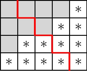
Recall that in $\mathrm{Gr}(2n+1,n)$, the Schubert varieties are indexed by partitions $\lambda$ whose Young diagram fit inside an $n\times (n+1)$ rectangle. Suppose we divide this rectangle into two staircases as shown below using the red cut, and only consider the partitions $\lambda$ that are symmetric with respect to the reflective map taking the upper staircase to the lower.

We claim that the Schubert varieties of the orthogonal Grassmannian are indexed by the ``shifted partitions’’ formed by ignoring the lower half of these symmetric partition diagrams. In fact, the Schubert varieties consist of the isotropic elements of the ordinary Schubert varieties, giving a natural embedding $\mathrm{OG}(2n+1,n)\to \mathrm{Gr}(2n+1,n)$ that respects the Schubert decompositions.

To get a sense of how this works, let’s look at the example of the partition $(4,3,1)$ shown above, in the case $n=4$. As described in this post, in the ordinary Grassmannian, the Schubert cell $\Omega_\lambda^{\circ}$ with respect to the standard flag is given by the set of vector spaces spanned by the rows of matrices whose reduced row echelon form looks like:

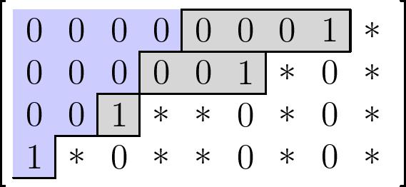
Combinatorially, this is formed by drawing the staircase pattern shown at the left, then adding the partition parts $(4,3,1)$ to it, and placing a $1$ at the end of each of the resulting rows for the reduced row echelon form.

Now, which of these spaces are isotropic? In other words, what is $\Omega_\lambda^{\circ}\cap \mathrm{OG}(2n+1,n)$? Well, suppose we label the starred entries as shown, where we have ommited the $0$’s to make the entries more readable:

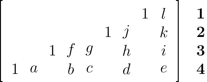
Then I claim that the entries $l,j,k,h,i,e$ are all uniquely determined by the values of the remaining variables $a,b,c,d,f,g$. Thus there is one isotropic subspace in this cell for each choice of values $a,b,c,d,f,g$, corresponding to the “lower half” of the partition diagram we started with:

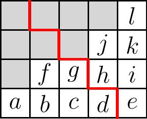
Indeed, let the rows of the matrix be labeled $\mathbf{1},\mathbf{2},\mathbf{3},\mathbf{4}$ from top to bottom as shown, and suppose its row span is isotropic. Since row $\mathbf{1}$ and $\mathbf{4}$ are orthogonal with respect to the reverse dot product, we get the relation \[l+a=0,\] which expresses $l=-a$ in terms of $a$.

Now, rows $\mathbf{2}$ and $\mathbf{4}$ are also orthogonal, which means that \[b+k=0,\] so we can similarly eliminate $k$. From rows $\mathbf{2}$ and $\mathbf{3}$, we obtain $f+j=0$, which expresses $j$ in terms of the lower variables. We then pair row $\mathbf{3}$ with itself to see that $h+g^2=0$, eliminating $h$, and finally pairing $\mathbf{3}$ with $\mathbf{4}$ we have $i+gc+d=0$, so $i$ is now expressed in terms of lower variables as well.

Moreover, these are the only relations we get from the isotropic condition - any other pairings of rows give the trivial relation $0=0$. So in this case the Schubert variety restricted to the orthogonal Grassmannian has half the dimension of the original, generated by the possible values for $a,b,c,d,f,g$.

General elimination argument

Why does this elimination process work in general, for a symmetric shape $\lambda$? Label the steps of the boundary path of $\lambda$ by $1,2,3,\ldots$ from SW to NE in the lower left half, and label them from NE to SW in the upper right half, as shown:

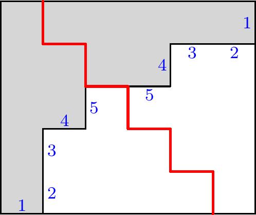
Then the labels on the vertical steps in the lower left half give the column indices of the $1$’s in the corresponding rows of the matrix. The labels on the horizontal steps in the upper half, which match these labels by symmetry, give the column indices from the right of the corresponding starred columns from right to left.

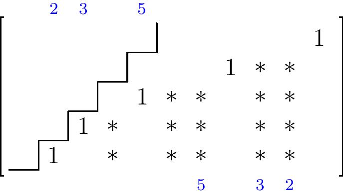
This means that the $1$’s in the lower left of the matrix correspond to the opposite columns of those containing letters in the upper right half. It follows that we can use the orthogonality relations to pair a $1$ (which is leftmost in its row) with a column entry in a higher or equal row so as to express that entry in terms of other letters to its lower left. The $1$ is in a lower or equal row in these pairings precisely for the entries whose corresponding square lies above the staircase cut. Thus we can always express the upper right variables in terms of the lower left, as in our example above.

Isotropic implies symmetric

We can now conversely show that if a point of the Grassmannian is isotropic, then its corresponding partition is symmetric about the staircase cut. Indeed, we claim that if the partition is not symmetric, then two of the $1$’s of the matrix will be in opposite columns, resulting in a nonzero reverse dot product between these two rows.

To show this, first note that we cannot have a $1$ in the middle column, for otherwise its row would not be orthogonal to itself. Therefore, of the remaining $2n$ columns, some $n$ of them have a $1$ in them, and the complementary columns must be the other $n$, the ones without a $1$. But this is the same combinatorial data as choosing some $k$ columns from the first $n$ columns, and the remaining columns being forced to be a pivot column if their opposite is not and vice versa. This implies that the partition is symmetric.

Coming soon: Combinatorics of shifted partitions and tableaux

From the above analysis, it follows that the orthogonal Grassmannian is partitioned into Schubert cells given by the data of a shifted partition, the upper half of a symmetric partition diagram:

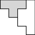
Such a partition is denoted by its distinct ``parts’’, the number of squares in each row, thought of as the parts of a partition with distinct parts shifted over by the staircase. For instance, the shifted partition above is denoted $(3,1)$.

The beauty of shifted partitions is that so much of the original tableaux combinatorics that goes into ordinary Schubert calculus works almost the same way for shifted tableaux and the orthogonal Grassmannian. We can define jeu de taquin, Knuth equivalence, and dual equivalence on shifted tableaux, there is a natural notion of a Littlewood-Richardson shifted tableau, and these notions give rise to formulas for both intersections of Schubert varieties in the orthogonal Grassmannian and to products of Schur $P$-functions or Schur $Q$-functions, both of which are specializations of the Hall-Littlewood polynomials.

I’ll likely go further into the combinatorics of shifted tableaux in future posts, but for now, I hope you enjoyed the breakdown of why shifted partitions are the natural indexing objects for the Schubert decomposition of the orthogonal Grassmannian.