Moduli of Curves IV: Getting classy

Young tableaux are to planes as labeled trees are to curves. Continuing from the previous post in this series, we now show how to think of $\overline{M}_{0,n}$ as a projective variety.

We now show how to look from the perspective of a single point, and combine this with the forgetting maps, to construct a projective embedding of $\overline{M}_{0,n}$ and thereby realize it as a geometric space itself, rather than just as a set of curves. The key new construction we need is the Kapranov map.

The Kapranov map

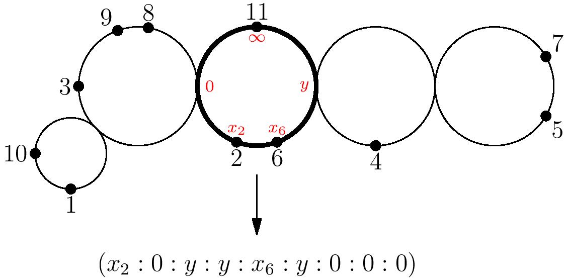
Given a curve $C\in \overline{M}_{0,n}$, consider the $\mathbb{P}^1$ component that the marked point $n$ is on. The other special points on this component are either nodes, each leading to a distinct branch of the dual tree, or marked points (which can be considered branches with just one leaf). Choose coordinates on this $\mathbb{P}^1$ in a way so that point $n$ is at coordinate $\infty=(1:0)$, and the branch containing marked point $1$ is attached at coordinate $0=(0:1)$. Then define the Kapranov map \[ \psi_n: \overline{M}_{0,n}\to \mathbb{P}^{n-3} \] that sends a curve $C$ to the tuple $(x_2:x_3:\cdots : x_{n-1})$ where $(x_i:1)$ is the coordinate at which the branch containing $i$ is attached to $n$’s component. (Note that this means that all $x_i$’s for $i$ in a given branch are equal.)

Essentially, $\psi_n$ contains all of, and only, the data of what the curve looks like from $n$’s perspective. It can “see” where the other branches are attached to its component, and it “knows” which points are on those branches, but it doesn’t know the tree structure or locations of the points out on those branches; it can only see its own line.

In particular, $\psi_n$ is a map to projective space, but it is not injective; by changing the structure out on the branches, we can have two different curves mapping to the same point under $\psi_n$:

Remarkably, we can fix the injectivity using the forgetting map.

Forgetting again

Recall that \[\pi_n:\overline{M}_{0,n}\to \overline{M}_{0,n-1} \] is the forgetting map that deletes the $n$th marked point (and collapsing its component to a point if there were only $3$ special points on the component containing $n$). For instance, applying $\pi_{11}$ to the first curve above yields:

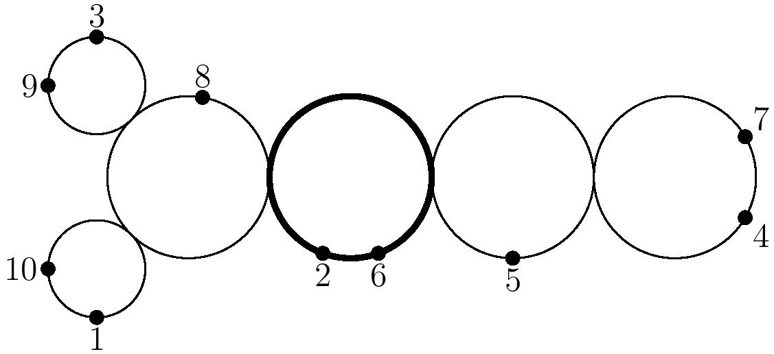
We claim that the data of $\pi_n(C)$, combined with $\psi_n(C)$, is enough to uniquely reconstruct the curve $C$. In other words:

Lemma. The map \[ \psi_n\times \pi_n : \overline{M}_{0,n} \to \mathbb{P}^{n-3} \times\overline{M}_{0,n-1}\] is injective (as a map of sets).

Proof. We wish to show that we can recover any curve $C$ uniquely from $\pi_n(C)$ and $\psi_n(C)$. Let $C’=\pi_n(C)$. Then $C$ must be formed from $C’$ by inserting the marked point $n$ somewhere on $C’$, including possibly colliding with another marked point and bubbling off, or colliding with a node, in which case the portions of the curve on each side of the node are separated and attached to a new line that also contains $n$.

If $C$ is formed from $C’$ by inserting $n$ at a non-special point on the curve, then the data of $\psi_n(C)$ will show which points are on the same branch as each other by looking at equalities among the coordinates, and so it will uniquely identify which component $n$ is inserted on. (For instance, if $x_4=x_5=x_7$ are all the coordinates of a given value, then there is a branch of the dual tree containing $4,5,7$ that is attached to the line containing $n$ by a node, thus uniquely determining the line containing $n$). Then, the coordinate values in $\psi_n(C)$ determine the location of $n$ on that line, relative to where the other branches are attached.

Similarly, if $C$ is formed by inserting $n$ in a way that collides with a special point, then $\psi_n(C)$ is a binary vector of $0$ and $1$ coordinates only, and again this determines the two branches that $n$ separates (or, if there is only one $1$, the marked point that $n$ collided with). This completes the proof. QED

Iterating to obtain a projective embedding

We now can iterate on $\overline{M}_{0,n-1}$ and so on, to get an injection into a product of projective spaces. For instance we have a chain of injections:

\[ \overline{M}_{0,6} \hookrightarrow \mathbb{P}^{3} \times\overline{M}_{0,5}\hookrightarrow \mathbb{P}^{3} \times \mathbb{P}^{2}\times \overline{M}_{0,4}\cong \mathbb{P}^{3} \times \mathbb{P}^{2}\times \mathbb{P}^1.\]

(We leave it as an exercise to the reader to show that $\psi_4$ is a bijection from $\overline{M}_{0,4}$ to $\mathbb{P}^1$.) This injection can technically be written as $\psi_6 \times (\psi_5\circ \pi_6) \times (\psi_4\circ \pi_5\circ \pi_6)$, but we think of it simply as the iterated Kapranov embedding.

Monin and Rana conjectured homogeneous equations that cut out the image of this embedding as a projective variety, and in joint work with Griffin and Levinson, we proved that the equations do indeed cut out $\overline{M}_{0,n}$ scheme-theoretically. This can be thought of as a parallel to the Plücker embedding of the Grassmannian, and in a simple example, we have that $\overline{M}_{0,5}$ is the subvariety of $\mathbb{P}^1\times \mathbb{P}^2$, say with coordinates $(u:v)\times (x:y:z)$, cut out by the single equation \[uy(x − z) = vx(y − z). \]

Thus, by combining the perspective and forgetting maps, we now have an elementary way of constructing $\overline{M}_{0,n}$ as a projective variety. Beautiful!